用户体验可视化指南pdf_R中增强可视化的初学者指南

用户体验可视化指南pdf

Learning to build complete visualizations in R is like any other data science skill, it’s a journey. RStudio’s ggplot2 is a useful package for telling data’s story, so if you are newer to ggplot2 and would love to develop your visualizing skills, you’re in luck. I developed a pretty quick — and practical — guide to help beginners advance their understanding of ggplot2 and design a couple polished, business-insightful graphs. Because early success with visualizations can be very motivating!

学习在R中构建完整的可视化效果就像其他任何数据科学技能一样，是一段旅程。 RStudio的ggplot2是一个有用的软件包，用于讲述数据的故事，因此，如果您是ggplot2的新手，并且希望发展自己的可视化技能，那么您会很幸运。 我开发了一个非常快速且实用的指南，以帮助初学者提高对ggplot2的理解，并设计一些精美的，具有业务洞察力的图表。 因为可视化的早期成功会非常有激励作用！

This tutorial assumes you have completed at least one introduction to ggplot2, like this one. If you haven’t, I encourage you to first to get some basics down.

本教程假定您至少已完成ggplot2的介绍， 例如本教程。 如果您还没有，我鼓励您首先了解一些基础知识。

By the end of this tutorial you will:

在本教程结束时，您将：

• Deepen your understanding for enhancing visualizations in ggplot2
  加深对ggplot2中可视化效果的理解
• Become familiar with navigating the ggplot2 cheat sheet (useful tool)
  熟悉导航ggplot2备忘单(有用的工具)
• Build two original, polished visuals shown below through a simple, step-by-step format
  通过简单的分步格式构建两个原始的，经过抛光的视觉效果，如下所示

Visualization #2

可视化＃2

Before we begin, here are a couple tools that can support your learning. The first is the ‘R Studio Data Visualization with ggplot2 cheat sheet’ (referred to as ‘cheat sheet’ from now on). We will reference it throughout to help you navigate it for future use.

在我们开始之前，这里有一些工具可以支持您的学习。 第一个是“带有ggplot2备忘单的R Studio数据可视化”(从现在开始称为“备忘单”)。 我们将始终引用它，以帮助您导航以备将来使用。

The second is a ‘ggplot2 Quick Guide’ I made to help me build ggplots on my own faster. It’s not comprehensive, but it may help you more quickly understand the big picture of ggplot2.

第二个是“ ggplot2快速指南 ” ，它旨在帮助我更快地自行构建ggplots。 它并不全面，但是可以帮助您更快地了解ggplot2的概况。

我们走吧！ (Let’s go!)

For this tutorial, we will use the IBM HR Employee Attrition dataset, available here. This data offers (fictitious) business insight and requires no preprocessing. Sweet!

在本教程中，我们将使用IBM HR Employee Attrition数据集 ， 可从此处获得 。 该数据提供(虚拟的)业务洞察力，不需要进行预处理。 甜！

Let’s install libraries and import the data.

让我们安装库并导入数据。

# install libraries
library(ggplot2)
library(scales)
install.packages("ggthemes") 
library(ggthemes)# import data
data <- read.csv(file.path('C:YourFilePath’, 'data.csv'), stringsAsFactors = TRUE)

Then check the data and structure.

然后检查数据和结构。

# view first 5 rows
head(attrition)# check structure
str(attrition)

Upon doing so, you will see that there are 1470 observations with 35 employee variables. Let’s start visual #1.

这样做之后，您将看到有1470个观察值和35个员工变量。 让我们开始视觉＃1。

视觉＃1 (Visual #1)

HR wants to know how monthly income is related to employee attrition by job role.

人力资源部想知道按职位 划分的月收入与员工流失之间的关系。

步骤1.数据，美学，几何 (Step 1. Data, Aesthetics, Geoms)

For this problem, ‘JobRole’ is our X variable (discrete) and ‘MonthlyIncome’ is our Y variable (continuous). ‘Attrition’ (yes/no) is our z variable.

对于此问题，“ JobRole”是我们的X变量(离散)，“ MonthlyIncome”是我们的Y变量(连续)。 “损耗”(是/否)是我们的z变量。

Check side 1 of your cheat sheet under ‘Two Variables: Discrete X, Continuous Y,’ and note the various graphs. We will use geom_bar(). On the cheat sheet, it’s listed as geom_bar(stat = ‘identity’). This would give us total monthly income of all employees. We instead want average, so we insert (stat = ‘summary’, fun = mean).

在“两个变量：离散X，连续Y”下检查备忘单的第一面，并记下各种图形。 我们将使用geom_bar()。 在备忘单上，它被列为geom_bar(stat ='identity')。 这将给我们所有雇员的总月收入。 相反，我们想要平均值，所以我们插入(stat ='summary'，fun = mean)。

# essential layers
ggplot(data, aes(x = JobRole, y = MonthlyIncome, fill=Attrition)) +
  geom_bar(stat = 'summary', fun = mean) #Gives mean monthly income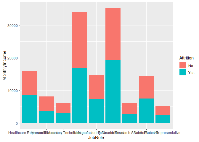

We obviously can’t read the names, which leads us to step 2…

我们显然无法读取名称，这导致我们进入步骤2…

步骤2.座标和位置调整 (Step 2. Coordinates and Position Adjustments)

When names are too long, it often helps to flip the x and y axis. To do so, we will add coord_flip() as a layer, as shown below. We will also unstack the bars to better compare Attrition, by adding position = ‘dodge’ within geom_bar() in the code. Refer to the ggplot2 cheat sheet side 2, ‘Coordinate Systems’ and ‘Position Adjustments’ to see where both are located.

名称太长时，通常有助于翻转x和y轴。 为此，我们将添加coord_flip()作为图层，如下所示。 通过在代码的geom_bar()中添加position ='dodge'，我们还将对这些条进行堆叠以更好地比较损耗。 请参考ggplot2备忘单第2面，“坐标系”和“位置调整”，以了解两者的位置。

# unstack bars and flipping axis
ggplot(data, aes(x = JobRole, y = MonthlyIncome, fill=Attrition)) +
  geom_bar(stat = ‘summary’, fun = mean, position = ‘dodge’) +
  coord_flip()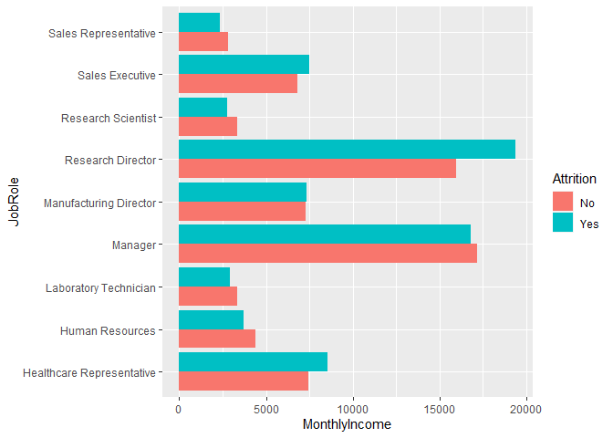

步骤3.从最高到最低重新排列条形 (Step 3. Reorder bars from highest to lowest)

Now, let’s reorder the bars from highest to lowest Monthly Income to help us better analyze by Job Role. Add the reorder code below within the aesthetics line.

现在，让我们从月收入的最高到最低重新排序，以帮助我们更好地按工作角色进行分析。 在美学行中的下方添加重新订购代码。

# reordering job role
ggplot(data, aes(x = reorder(JobRole, MonthlyIncome), y = MonthlyIncome, fill = Attrition)) +
  geom_bar(stat = 'summary', fun = mean, position = 'dodge') +
  coord_flip()

步骤4.更改条形颜色和宽度 (Step 4. Change bar colors and width)

Let’s change the bar colors to “match the company brand.” This must be done manually, so find scale_fill_manual() on side 2 of the cheat sheet, under “Scales.” It lists colors in base R. You can try some, but they aren’t “company colors.” I obtained the color #s below from color-hex.com.

让我们更改条形颜色以“匹配公司品牌”。 这必须手动完成，因此请在备忘单第二侧的“比例”下找到scale_fill_manual()。 它在基准R中列出了颜色。您可以尝试一些，但它们不是“公司颜色”。 我从color-hex.com获得以下颜色＃。

Also, we will narrow the bar widths by adding ‘width=.8’ within geom_bar() to add visually-appealing space.

另外，我们将通过在geom_bar()中添加'width = .8'来缩小条形宽度，以增加视觉上吸引人的空间。

ggplot(data, aes(x = reorder(JobRole, MonthlyIncome), y = MonthlyIncome, fill = Attrition)) +
  geom_bar(stat='summary', fun=mean, width=.8, position='dodge') +
  coord_flip() +
  scale_fill_manual(values = c('#96adbd', '#425e72'))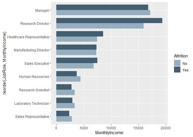

步骤5.标题和轴标签 (Step 5. Title and Axis Labels)

Now let’s add Title and Labels. We don’t need an x label since the job titles explain themselves. See the code for how we handled. Also, check out “Labels” on side 2 of the cheat sheet.

现在让我们添加标题和标签。 我们不需要x标签，因为职位说明了自己。 请参阅代码以了解我们的处理方式。 另外，请检查备忘单第二面的“标签”。

ggplot(data, aes(x = reorder(JobRole, MonthlyIncome), y = MonthlyIncome, fill = Attrition)) +
  geom_bar(stat='summary', fun=mean, width=.8, position='dodge') +
  coord_flip() +
  scale_fill_manual(values = c('#96adbd', '#425e72')) +
  xlab(' ') +  #Removing x label
  ylab('Monthly Income in USD') +
  ggtitle('Employee Attrition by Job Role & Income')

步骤6.添加主题 (Step 6. Add Theme)

A theme will kick it up a notch. We will add a theme layer at the end of our code, as shown below. When you start typing ‘theme’ in R, it shows options. For this graph, I chose theme_clean()

一个主题将使它提升一个等级。 我们将在代码末尾添加一个主题层，如下所示。 当您开始在R中键入“主题”时，它会显示选项。 对于此图，我选择了theme_clean()

#Adding theme after title
ggtitle('Employee Attrition by Job Role & Income') +
  theme_clean()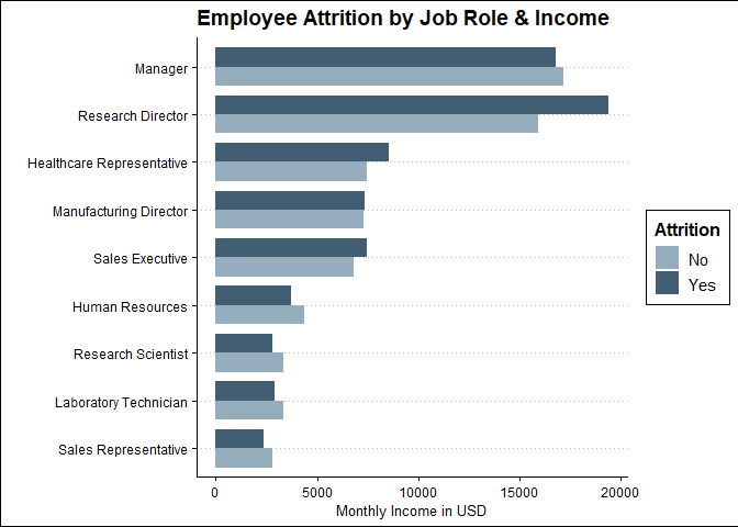

步骤7.降低图形高度并使轮廓不可见 (Step 7. Reduce graph height and make outlines invisible)

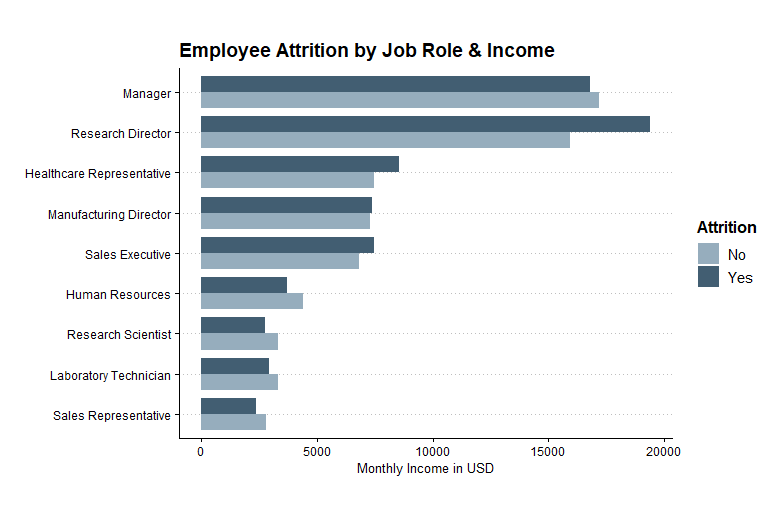
Just two easy tweaks. First, we will remove the graph and legend outlines. Second, the graph seems tall, so let’s reduce the height via aspect.ratio within theme(). Here is the full code for the final graph.

只需两个简单的调整。 首先，我们将删除图形和图例轮廓。 其次，图形看起来很高，因此让我们通过theme()中的Aspect.ratio降低高度。 这是最终图形的完整代码。

ggplot(data, aes(x = reorder(JobRole, MonthlyIncome), y = MonthlyIncome, fill = Attrition)) +
  geom_bar(stat='summary', fun=mean, width=.8, position='dodge') +
  coord_flip() +
  scale_fill_manual(values = c('#96adbd', '#425e72')) +
  xlab(' ') +
  ylab('Monthly Income in USD') +
  ggtitle('Employee Attrition by Job Role & Income') +
  theme_clean() +
  theme(aspect.ratio = .65,
    plot.background = element_rect(color = 'white'),
    legend.background = element_rect(color = 'white'))

Nice. We see that Research Directors who make more in monthly income are more likely to leave the company. The opposite is the case for other job roles.

真好 我们发现，月收入更高的研究主管更有可能离开公司。 其他工作角色则相反。

You’ve accomplished a lot. Ready for another go? Visual 2 walk-through will be a piece of cake.

您已经取得了很多成就。 准备再去吗？ Visual 2演练将是小菜一碟。

视觉＃2 (Visual #2)

For the second visual, we want to know if employee attrition has any relationship to monthly income, years since last promotion, and work-life balance. Another multivariate analysis.

对于第二个视觉图像，我们想知道员工的流失是否与月收入 ， 自上次升职以来 的年限以及工作与生活的平衡有关。 另一个多元分析。

步骤1.数据，美学，几何 (Step 1. Data, Aesthetics, Geoms)

For this problem, ‘MonthlyIncome’ is our X and ‘YearsSinceLastPromotion’ is our Y variable. Both are continuous, so check side 1 of your cheat sheet under ‘Two Variables: Continuous X, Continuous Y.’ For visualization context, we will use geom_smooth(), a regression line often added to scatter plots to reveal patterns. ‘Attrition’ will again be differentiated by color.

对于此问题，“ MonthlyIncome”是我们的X，“ YearsSinceLastPromotion”是我们的Y变量。 两者都是连续的，因此请检查备忘单第1面的“两个变量：连续X，连续Y”。 对于可视化上下文，我们将使用geom_smooth()，这是一条通常添加到散点图中以揭示模式的回归线。 “损耗”将再次通过颜色区分。

ggplot(data, aes(x=MonthlyIncome, y=YearsSinceLastPromotion, color=Attrition)) +
  geom_smooth(se = FALSE) #se = False removes confidence shading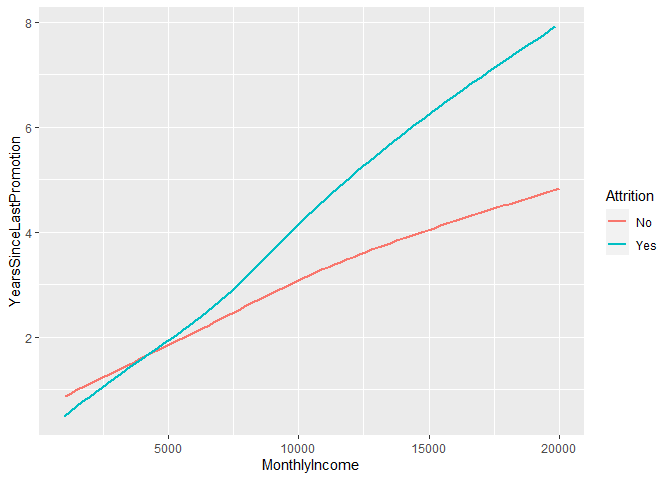

We can see that employees who leave are promoted less often. Let’s delve deeper and compare by work-life balance. For this 4th variable, we need to use ‘Faceting’ to view subplots by work-life balance level.

我们可以看到，离职的员工升职的频率降低了。 让我们深入研究并通过工作与生活之间的平衡进行比较。 对于第四个变量，我们需要使用“ Faceting”以按工作与生活的平衡水平查看子图。

步骤2.刻面将子图添加到画布 (Step 2. Faceting to add subplots to the canvas)

Check out ‘Faceting’ on side 2 of the cheat sheet. We will use facet_wrap() for a rectangular layout.

检查备忘单第二面的“ Faceting”。 我们将facet_wrap()用于矩形布局。

ggplot(data, aes(x = MonthlyIncome, y = YearsSinceLastPromotion, color=Attrition)) +
  geom_smooth(se = FALSE) +
  facet_wrap(WorkLifeBalance~.)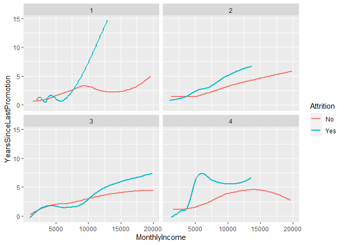

The facet grids look good, but what do the numbers mean? The data description explains the codes for ‘WorkLifeBalance’: 1 = ‘Bad’, 2 = ‘Good’, 3 = ‘Better’, 4 = ‘Best’. Add them in step 3.

刻面网格看起来不错，但是数字意味着什么？ 数据说明解释了“ WorkLifeBalance”的代码：1 =“差”，2 =“好”，3 =“更好”，4 =“最好”。 在步骤3中添加它们。

步骤3.将标签添加到构面子图 (Step 3. Add Labels to Facet Subplots)

To add subplot labels, we need to first define the names with a character vector, then use the ‘labeller’ function within facet_wrap.

要添加子图标签，我们需要首先使用字符向量定义名称，然后在facet_wrap中使用'labeller'函数。

# define WorkLifeBalance values
wlb.labs <- c('1' = 'Bad Balance', '2' = 'Good Balance', '3' = 'Better Balance', '4' = 'Best Balance')#Add values to facet_wrap()
ggplot(data, aes(x = MonthlyIncome, y = YearsSinceLastPromotion, color=Attrition)) +
  geom_smooth(se = FALSE) +
  facet_wrap(WorkLifeBalance~., 
    labeller = labeller(WorkLifeBalance = wlb.labs))

步骤4.标签和标题 (Step 4. Labels and Title)

Add your labels and title at the end of your code.

在代码末尾添加标签和标题。

facet_wrap(WorkLifeBalance~.,
    labeller = labeller(WorkLifeBalance = wlb.labs)) +
xlab('Monthly Income') +
ylab('Years Since Last Promotion') +
ggtitle('Employee Attrition by Workplace Factors')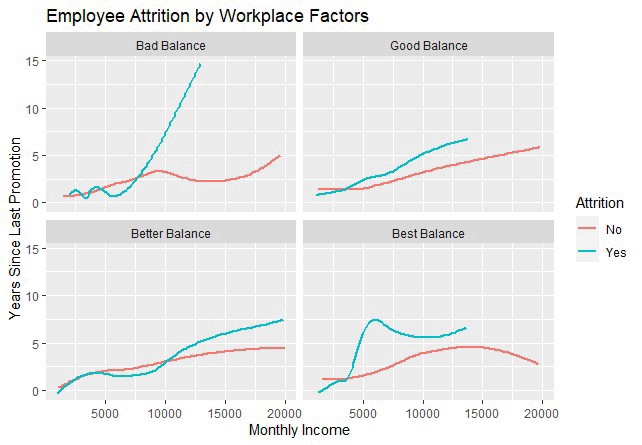

步骤5.在标签和刻度标记之间添加空格 (Step 5. Add Space Between Labels and Tick Markers)

When I look at the graph, the x and y labels seem too close to the tick markers. A simple trick is to insert newline (\n) code within label names.

当我查看图表时，x和y标签似乎太靠近刻度线标记。 一个简单的技巧是在标签名称中插入换行(\ n)代码。

xlab('\nMonthly Income') +  #Adds space above label
ylab('Years Since Last Promotion\n')  #Adds space below label

步骤6.主题 (Step 6. Theme)

When you installed library(‘ggthemes’), it gave you more options. For a modern look, I went with theme_fivethirtyeight(). Simply add at the end.

当您安装库('ggthemes')时，它为您提供了更多选择。 对于现代外观，我选择了theme_fivethirtyeight()。 只需在末尾添加即可。

ggtitle('Employee Attrition by Workplace Factors') +
  theme_fivethirtyeight()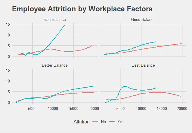

步骤7.覆盖主题默认值 (Step 7. Override a Theme Default)

What happened to our x and y labels? Well, the default for theme_fivethirtyeight() doesn’t have labels. But we can easily override that with a second theme() layer at the end of your code as shown below.

我们的x和y标签发生了什么？ 好吧，theme_fivethirtyeight()的默认值没有标签。 但是我们可以在代码末尾的第二个theme()层轻松覆盖它，如下所示。

theme_fivethirtyeight() +
theme(axis.title = element_text())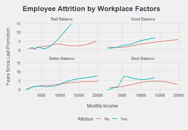

Not bad. But…people may not be able to tell if ‘Better Balance’ and ‘Best Balance’ are for the top or bottom grids right away. Let’s also change our legend location in step 8.

不错。 但是……人们可能无法立即判断出“最佳平衡”和“最佳平衡”是用于顶部还是底部网格。 我们还要在步骤8中更改图例位置。

步骤8.在网格之间添加空间并更改图例位置 (Step 8. Add Space Between Grids and Change Legend Location)

Adding space between top and bottom grids and changing the legend location both occur within the second theme() line. See side 2 of cheat sheet under ‘Legends.’

在顶部和底部网格之间添加空间并更改图例位置都在第二个theme()行内。 请参阅“传奇”下备忘单的第二面。

theme_fivethirtyeight() +
theme(axis.title = element_text(),
  legend.position = 'top',
  legend.justification = 'left',
  panel.spacing = unit(1.5, 'lines'))

步骤9。更改线条颜色 (Step 9. Change Line Color)

It would be awesome to change line colors to pack a visual punch. Standard R colors don’t quite meet our needs. We will change manually just like we did with Visual #1. I obtained the colors #s from color-hex.com, which has become a useful tool for us.

更改线条颜色以增加视觉冲击力真是太棒了。 标准R颜色不能完全满足我们的需求。 我们将像使用Visual＃1一样手动进行更改。 我从color-hex.com获得了颜色＃，它已成为我们的有用工具。

Here is the full code for the second visual.

这是第二个视觉效果的完整代码。

ggplot(data, aes(x = MonthlyIncome, y = YearsSinceLastPromotion, color=Attrition)) +
  geom_smooth(se = FALSE) +
  facet_wrap(WorkLifeBalance~., 
    labeller = labeller(WorkLifeBalance = wlb.labs)) +
  xlab('\nMonthly Income') +  
  ylab('Years Since Last Promotion\n') +
  theme_ggtitle('Employee Attrition by Workplace Factors') +
  theme_fivethirtyeight() +
  theme(axis.title = element_text(),
    legend.position = 'top',
    legend.justification = 'left',
    panel.spacing = unit(1.5, 'lines')) +
  scale_color_manual(values = c('#999999','#ffb500'))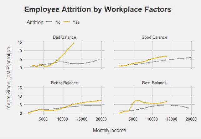

Another job well done. We see that employees in roles lacking work-life balance seem to stay if promotions are more frequent. The difference in attrition is less noticeable in good or higher work-life balance levels.

另一项工作做得很好。 我们看到，如果升职更加频繁，则缺乏工作与生活平衡的角色的员工似乎会留下来。 在良好或较高的工作与生活平衡水平下，损耗的差异不太明显。

In this tutorial, we gained skills needed for ggplot2 visual enhancement, became more familiar with the R Studio ggplot2 cheat sheet, and built two nice visuals. I hope that the step-by-step explanations and cheat sheet referencing were helpful and enhanced your confidence using ggplot2.

在本教程中，我们获得了ggplot2视觉增强所需的技能，对R Studio ggplot2备忘单更加熟悉，并构建了两个不错的视觉效果。 我希望逐步说明和备忘单参考对您有所帮助，并使用ggplot2增强您的信心。

Many are helping me as I advance my data science and machine learning skills, so my goal is to help and support others in the same way.

随着我提高数据科学和机器学习技能，许多人正在帮助我，所以我的目标是以同样的方式帮助和支持他人。

翻译自: https://towardsdatascience.com/beginners-guide-to-enhancing-visualizations-in-r-9fa5a00927c9

用户体验可视化指南pdf