


A man is walking a dog on a leash: the man can move on one curve, the dog on the other; both may vary their speed, but backtracking is not allowed. What is the length of the shortest leash that is sufficient for traversing both curves? [1]
一个人用皮带walking狗:该人可以在一条曲线上移动,而狗则可以在另一条曲线上移动。 两者都可能改变速度,但是不允许回溯。 足以横贯两条曲线的最短牵引带的长度是多少? [1]
The above quote helps develop the intuition for the definition of the Fréchet distance between two curves. Its discrete counterpart measures the similarity between two directed polygonal lines, defined as sets of connected points in some metric space. In an oriented polygonal line, the sequence of vertices is of interest and describes a direction, like a vehicle’s trajectory. Other similarity measures like the Hausdorff distance are oblivious of the line orientation and yield a high similarity for polygonal lines with close vertices, but with the reverse direction.
上面的引用有助于发展直觉,以定义两条曲线之间的Fréchet距离。 它的离散对应物测量两条有向折线之间的相似度,这两条折线定义为某些度量空间中的连接点集。 在定向的折线中,顶点序列令人感兴趣,并描述了方向,例如车辆的轨迹。 其他相似性度量(如Hausdorff距离)会忽略线的方向,并且会为具有近似顶点但方向相反的多边形线提供高度相似性。
I already described this similarity metric in another article, where I discussed the original implementation based on dynamic programming. I provided a speed-optimized version by linearizing the algorithm (by replacing recursion with two nested loops), which improved performance almost tenfold. Although the new upgraded algorithm runs faster, it still consumes the same amount of memory, which is undesirable for very large polylines.
我已经在另一篇文章中描述了这种相似性度量,其中讨论了基于动态编程的原始实现。 我通过线性化算法(通过用两个嵌套循环替换递归)提供了速度优化的版本,将性能提高了近十倍。 尽管新的升级算法运行速度更快,但仍消耗相同数量的内存,这对于很大的折线来说是不希望的。
This article provides two alternative implementations of the same algorithm containing performance improvements according to a set of recent papers [2, 3]. The first implementation uses linear arrays to store the data while the second uses a sparse array based on a dictionary for very large polylines. All code is JIT-compiled using the Numba package for top performance.
本文根据一组最新论文[2,3]提供了相同算法的两种替代实现,其中包含性能改进。 第一种实现使用线性数组存储数据,而第二种实现使用基于字典的稀疏数组来存储非常大的折线。 使用Numba软件包对所有代码进行JIT编译,以实现最佳性能。
逻辑优化 (Logic Optimizations)
As I previously described, calculating the discrete Fréchet distance (DFD) involves building up a rectangular matrix with dimensions corresponding to the number of points in each polyline. The original dynamic programming algorithm fills up the whole array by performing a distance calculation for each element. It then compares the distance to the recursively calculated values for its neighbors to the left and top. It is clear that the larger the polylines are, the longer the algorithm takes to compute the matrix.
如前所述,计算离散弗雷歇距离(DFD)涉及建立一个矩形矩阵,其尺寸与每个折线中的点数相对应。 原始的动态编程算法通过对每个元素执行距离计算来填充整个数组。 然后,将距离与左侧和顶部的邻居的递归计算值进行比较。 显然,折线越大,算法计算矩阵所需的时间就越长。
We can make the algorithm run faster by reducing the number of points in each polyline through a line simplification algorithm, like the famous Ramer-Douglas-Peucker algorithm. I have used this algorithm in the past to help me display very large trajectories on a map. It works by removing points from the polyline while keeping its overall shape. The user gets the same information while the map display software avoids handling useless vertices, thereby improving performance and responsiveness. I will not explore this optimization here and will do so in a future article.
我们可以通过线简化算法减少每条折线中的点数,从而使算法运行更快,就像著名的Ramer-Douglas-Peucker算法一样。 过去,我曾使用此算法来帮助我在地图上显示非常大的轨迹。 它通过从折线中删除点同时保持其整体形状来工作。 当地图显示软件避免处理无用的顶点时,用户将获得相同的信息,从而提高了性能和响应速度。 我将不在这里探讨这种优化,并且将在以后的文章中进行探讨。
Another optimization lies buried deep in the DFD calculation mathematics and is similar to the “warping window” concept associated with Dynamic Time Warping. We only need to calculate some of the matrix elements close to the main diagonal as it turns out. By not calculating all the other items, we gain not only speed but can also save memory on very large polylines. This optimization also implies that we must consider a different data structure to store the matrix, possibly a sparse array. Besides avoiding the calculation of unnecessary data, we also do not allocate unneeded memory.
另一个优化方法深深地扎根于DFD计算数学中,类似于与动态时间规整相关的“规整窗口”概念。 事实证明,我们只需要计算一些靠近主对角线的矩阵元素。 通过不计算所有其他项,我们不仅可以提高速度,还可以节省很大的折线上的内存。 这种优化还意味着我们必须考虑不同的数据结构来存储矩阵,可能是稀疏数组。 除了避免计算不必要的数据外,我们也不会分配不需要的内存。
The optimization idea becomes evident if you look at a fully calculated matrix. To see this at work, let us look at an example. We will calculate the DFD for two polylines defined in a euclidean space.
如果您查看一个完全计算的矩阵,则优化思想将变得显而易见。 为了了解这一点,让我们来看一个例子。 我们将计算在欧式空间中定义的两条折线的DFD。
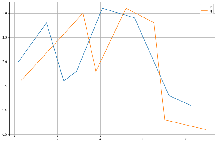
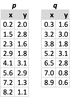
The polyline coordinates are as follows.
折线坐标如下。
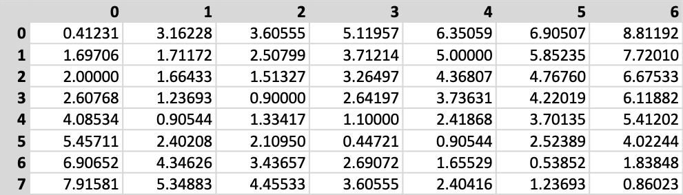
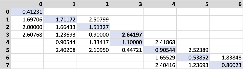
Now, we can calculate the distance matrix between both polylines. Note that this step will not fully occur during algorithm execution. I use it here for illustrations purposes only, as it clearly illustrates how values tend to increase as you move further away from the diagonal. The improved algorithm explores this feature to reduce the number of calculations and required storage.
现在,我们可以计算两条折线之间的距离矩阵。 请注意,此步骤在算法执行期间不会完全发生。 我在这里仅将其用于说明目的,因为它清楚地说明了当您进一步远离对角线时值如何趋于增加。 改进的算法探索了此功能,以减少计算量和所需的存储量。
We start by considering the diagonal cells only, but while it is quite simple to define on a square matrix, the diagonal of a rectangular matrix requires more work. Instead of the paper’s approach, I decided to revisit an old friend, Bresenham’s line drawing algorithm. If you think of a matrix as a raster display, the usefulness of the algorithm becomes obvious. Instead of using the algorithm to draw lines, I use it to generate pairs of matrix indices to connect the top left-hand corner with the lower right-hand corner.
我们仅从对角线单元开始,但是在方矩阵上定义非常简单,而矩形矩阵的对角线则需要更多工作。 我决定改用老朋友布雷森汉姆(Bresenham)的线条绘制算法,而不是论文的方法。 如果您将矩阵视为栅格显示,则该算法的用途变得显而易见。 我没有使用该算法绘制线条,而是使用它来生成矩阵索引对,以将左上角与右下角连接起来。
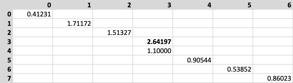
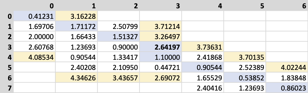
After calculating the diagonal, we take its maximum value as a top limit for the final distance. The algorithm proceeds by iterating through the diagonal left to right, and for each column, calculates the distances and stores them if they are smaller than the reference maximum. The same process applies to rows. The next figure depicts the result as pertains to this case. I have highlighted the diagonal with a light blue background for ease of reading.
计算对角线后,我们将其最大值作为最终距离的上限。 该算法通过从左到右迭代对角线进行,对于每一列,计算距离并存储距离(如果距离小于参考最大值)。 相同的过程适用于行。 下图描述了与此案例有关的结果。 为了方便阅读,我用浅蓝色背景突出显示了对角线。
It is relatively easy to see how much memory we have saved. Instead of the expected 42 items, we have only stored 26 of them. Still, we calculated more distances than we have kept, and this is depicted in the next figure.
比较容易看出我们节省了多少内存。 而不是预期的42个项目,我们仅存储了26个项目。 尽管如此,我们计算出的距离比我们保持的要多,下图对此进行了描述。
We cannot resort to the traditional NumPy arrays to save RAM, as these will allocate unnecessary memory. Here we will use a dictionary-based sparse matrix, and I will discuss its implementation details below along with the code optimization.
我们不能求助于传统的NumPy数组来节省RAM,因为它们会分配不必要的内存。 在这里,我们将使用基于字典的稀疏矩阵,下面将与代码优化一起讨论其实现细节。
We are now ready to move on to the second step, where the final calculations take place. First, we must create a new matrix, the Fréchet matrix, to store the final results. The process starts by copying the distance diagonal data into the Fréchet matrix. Next, we iterate each distance matrix element starting at the diagonal and apply a simple algorithm that calculates the final Fréchet cell value.
现在,我们准备进行第二步,在此进行最终计算。 首先,我们必须创建一个新的矩阵Fréchet矩阵,以存储最终结果。 该过程开始于将距离对角线数据复制到Fréchet矩阵中。 接下来,我们迭代从对角线开始的每个距离矩阵元素,并应用一种简单的算法来计算最终的Fréchet像元值。

The final calculation proceeds along with the distance matrix diagonal. Once finished, the Fréchet matrix looks like the following image.
最终计算与距离矩阵对角线一起进行。 完成后,Fréchet矩阵如下图所示。
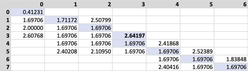
Please note that one can do away with the second matrix (F) and perform all calculations using just the distance matrix (D) due to how computation proceeds. As always, the final distance value is in the lower right-hand corner cell.
请注意,由于计算的进行方式,因此可以取消第二个矩阵(F)并仅使用距离矩阵(D)执行所有计算。 与往常一样,最终距离值位于右下角的单元格中。
代码优化 (Code Optimizations)
You can find all the code for this article in its GitHub repository. Besides the DFD’s original implementations, the code now contains two additional ones based on the paper’s insights. For smaller polylines, you can use the NumPy array-based version named FastDicreteFrechetMatrix. For larger polylines, you should probably use the sparse array version, called FastDiscreteFrechetSparse. This last version uses a dictionary to simulate a sparse array.
您可以在其GitHub存储库中找到本文的所有代码。 除了DFD的原始实现之外,该代码现在还包含两个基于本文见解的实现。 对于较小的折线,可以使用名为FastDicreteFrechetMatrix的基于NumPy数组的版本。 对于较大的折线,您可能应该使用称为FastDiscreteFrechetSparse的稀疏数组版本。 最新版本使用字典来模拟稀疏数组。
Most of the code is now JIT-compiled using Numba for dramatically increased performance. This package targets scientific computing code and understands most of NumPy, making your code lightning fast. There are a couple of things to watch out for when using Numba.
现在,大多数代码都使用Numba进行了JIT编译,以显着提高性能。 该软件包以科学计算代码为目标,并且了解NumPy的大多数内容,使您的代码闪电般快速。 使用Numba时需要注意几件事。
The first thing you will notice is the slow first-time execution of your compiled code. This delay occurs due to the JIT phase of compilation, where your Python code translates into machine code. All subsequent runs will be at full speed.
您会注意到的第一件事是编译后的代码第一次执行缓慢。 由于编译的JIT阶段而发生此延迟,在此阶段,您的Python代码转换为机器代码。 所有后续运行将全速运行。
The second issue with Numba is that it requires some getting used to because of compatibility issues with Python and NumPy. Not all your code will work, and when it does, it might not improve performance-wise. You should thoroughly read the package’s documentation to get the most of it. When you understand how to use it, Numba is a joy.
Numba的第二个问题是,由于Python和NumPy的兼容性问题,它需要一些习惯。 并非您的所有代码都能正常工作,并且当它运行时,可能无法提高性能。 您应该仔细阅读软件包的文档以充分利用它。 当您了解如何使用它时,Numba就是一种喜悦。
性能 (Performance)
To get a sense of how these algorithms perform, I set up a Jupyter notebook that compares two sets of trajectories (please see the accompanying code). The first set is relatively small, with 91 and 107 points, and the second is a bit larger, with 263 and 477 points. The code exercises all four algorithms against these two sets, as you can see by going through the notebook.
为了了解这些算法的性能,我建立了一个Jupyter笔记本,该笔记本比较了两组轨迹(请参见随附的代码)。 第一组相对较小,为91和107点,第二组较大,为263和477点。 如通过笔记本所看到的,该代码针对这两个集合使用了所有四种算法。
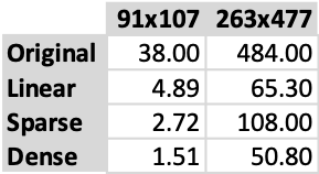
As you can expect, the original recursive algorithm is always the slowest by a large margin. Next up is its linear adaptation that runs considerably faster (an order of magnitude). Then we have mixed results from the sparse implementation of the improved algorithm. It runs faster than the previous two in the smaller set but slower on the larger. This performance difference is due to the sparse array implementation based on a dictionary — it does not scale well. A future revision of this code will focus on replacing this component with a more performant one, although it is still not clear what that might be. Finally, the array-based implementation of the improved algorithm is consistently faster.
如您所料,原始递归算法始终是最慢的。 接下来是它的线性自适应,运行速度相当快(一个数量级)。 然后,我们混合了改进算法的稀疏实现的结果。 它在较小的集合中比前两个运行得更快,但是在较大的集合中运行得慢。 这种性能差异是由于基于字典的稀疏数组实现导致的-扩展性不佳。 该代码的未来修订版将着重于用性能更高的组件替换该组件,尽管目前尚不清楚这可能是什么。 最后,改进算法的基于数组的实现始终更快。
It seems that, with the current implementation, we will have to strike a compromise between speed and size. For very large polylines, we will have to use a slower-performing algorithm, unfortunately. Hopefully, this will improve in the future.
看来,在当前的实现中,我们将不得不在速度和大小之间取得折衷。 不幸的是,对于很大的折线,我们将不得不使用性能较慢的算法。 希望将来会有所改善。
结论 (Conclusion)
This article reviewed a performance improvement to the discrete Fréchet distance using a recent paper’s results. Instead of having to calculate all the distance pairs, we can focus on a limited set of cells around the distance matrix diagonal. This approach not only saves space but also improves performance.
本文使用最新论文的结果对离散Fréchet距离的性能改进进行了回顾。 不必计算所有距离对,我们可以专注于距离矩阵对角线周围有限的一组像元。 这种方法不仅节省空间,而且提高了性能。
In a future article, I will illustrate the use of the discrete Fréchet distance in trajectory clustering. Each item to aggregate is a geospatial trajectory defined by a variable number of locations, and the DFD is the distance measure of choice for such a scenario. The performance improvements put forward in this article will no doubt be of use there.
在以后的文章中,我将说明离散Fréchet距离在轨迹聚类中的使用。 要聚合的每个项目都是由可变数量的位置定义的地理空间轨迹,而DFD是这种情况下选择的距离度量。 毫无疑问,本文中提出的性能改进将在这里有用。
翻译自: https://towardsdatascience.com/fast-discrete-fr%C3%A9chet-distance-d6b422a8fb77


 1万+
1万+

 被折叠的 条评论
为什么被折叠?
被折叠的 条评论
为什么被折叠?
 到【灌水乐园】发言


