马斯克神经网络转换器_神经网络动画转换数据

马斯克神经网络转换器

When it comes to classification algorithms, the explanation can be intuitive about how they work:

关于分类算法，可以很直观地说明它们的工作方式：

• Logistic Regression and SVM find a hyperplane to “cut” the space into two. (But the approach of these two algorithms is different, so the final hyperplane is different.)

  Logistic回归和SVM可以找到一个超平面将空间“切”为两个。 (但是这两种算法的方法不同，因此最终的超平面是不同的。)

• In case the data are not linearly separable, with the kernel trick, SVM transforms the data into a space of higher dimension, then “cuts” it into two.

  如果数据不是线性可分离的，则使用内核技巧， SVM将数据转换为高维空间，然后将其“切”为两部分。

• Decision trees group data into hyper-rectangles that will contain a majority of one class.

  决策树将数据分组为超矩形，它将包含一个类的大部分。

• K Nearest-Neighbors analyses the neighbors of a new observation to predict the class of this one.

  K最近邻居分析一个新观测值的邻居，以预测该观测值的类别。

Now what about Neural Network?

现在神经网络呢？

转换隐藏层 (Transformation of a hidden layer)

Let’s take a simple example of dataset: two classes, two features x1 and x2, and the data are not linearly separable.

让我们以一个简单的数据集示例为例：两个类，两个特征x1和x2，并且数据不是线性可分离的。

import numpy as npnp.random.seed(1)x1=np.concatenate((np.random.normal(0.5,0.1,100),
np.random.normal(0.2,0.05,50),
np.random.normal(0.8,0.05,50))).reshape(-1,1)x2=np.concatenate((np.random.normal(0.5,0.2,100),
np.random.normal(0.5,0.2,50),
np.random.normal(0.5,0.2,50))).reshape(-1,1)X=np.hstack((x1,x2))y=np.concatenate((np.repeat(0,100),np.repeat(1,100)))

The visualization is below and the data are also normalized.

可视化内容在下面，数据也已标准化。

from sklearn.preprocessing import StandardScaler
scaler = StandardScaler()
X=scaler.fit_transform(X)plt.scatter(X[:, 0], X[:, 1], c=y,s=20)
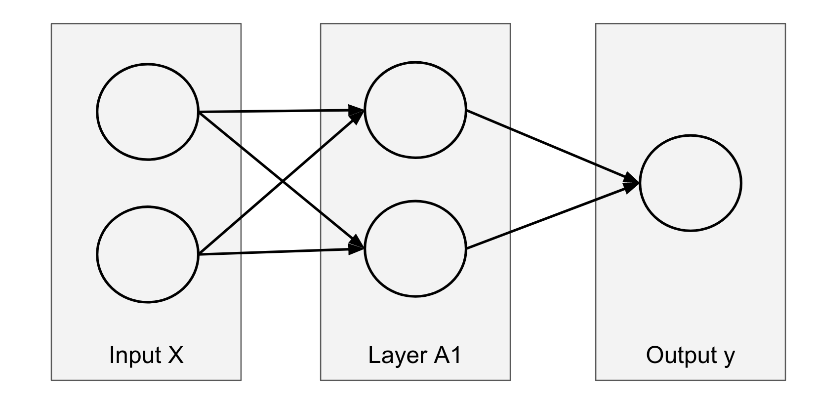
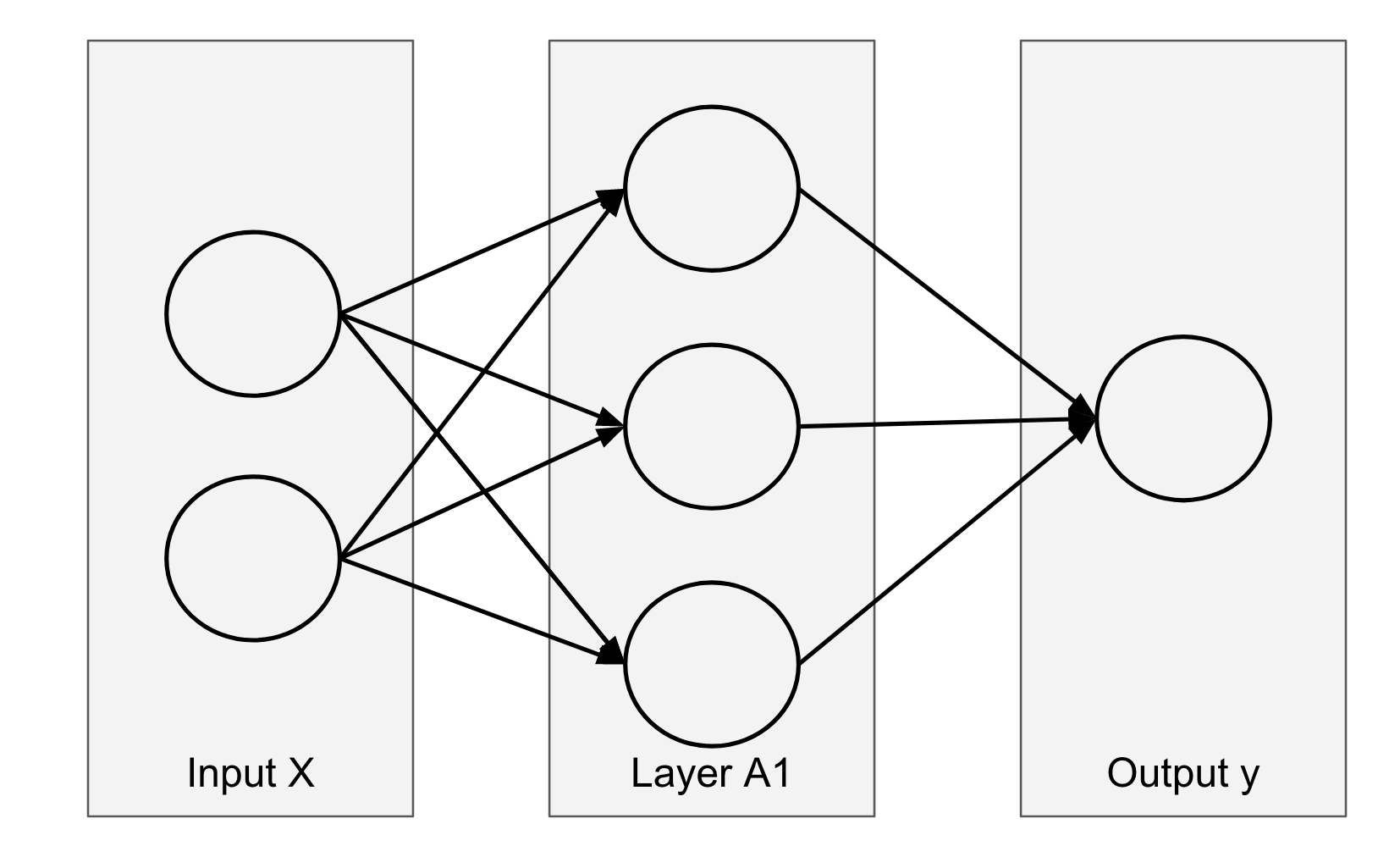
plt.axis('equal')

For this dataset, the simplest suitable structure of the neural network is the one with one hidden layer of two neurons. If you don’t see why, just continue and you will understand intuitively.

对于此数据集，神经网络最简单的合适结构是具有两个神经元的一个隐藏层的结构。 如果您不明白为什么，请继续，您将直观地理解。

We can also considerer that the activation function is the sigmoid function.

我们还可以考虑激活函数是S型函数。

from sklearn.neural_network import MLPClassifierclf = MLPClassifier(solver=’lbfgs’,hidden_layer_sizes=(2,),
activation=”logistic”,max_iter=1000)clf.fit(X, y)

The initial data are transformed by the hidden layer. Since the hidden layer has two neurons, we can visualize the outputs of the two neurons on a 2D plane.

初始数据由隐藏层转换。 由于隐藏层具有两个神经元，因此我们可以在二维平面上可视化两个神经元的输出。

So the initial 2D dataset is transformed into another 2D space.

因此，初始2D数据集将转换为另一个2D空间。

We can calculate the values of the hidden layer A1 with the corresponding weights:

我们可以使用相应的权重来计算隐藏层A1的值：

A1=1/(1+np.exp(-(X@clf.coefs_[0]+clf.intercepts_[0])))

Then we can visualize the layer A1:

然后我们可以可视化A1层：

fig, ax = plt.subplots(figsize=(5,5))
ax.scatter(A1[:, 0], A1[:, 1], c=y,s=30)
ax.set_xlim(-0.1, 1.1)
ax.set_ylim(-0.1, 1.1)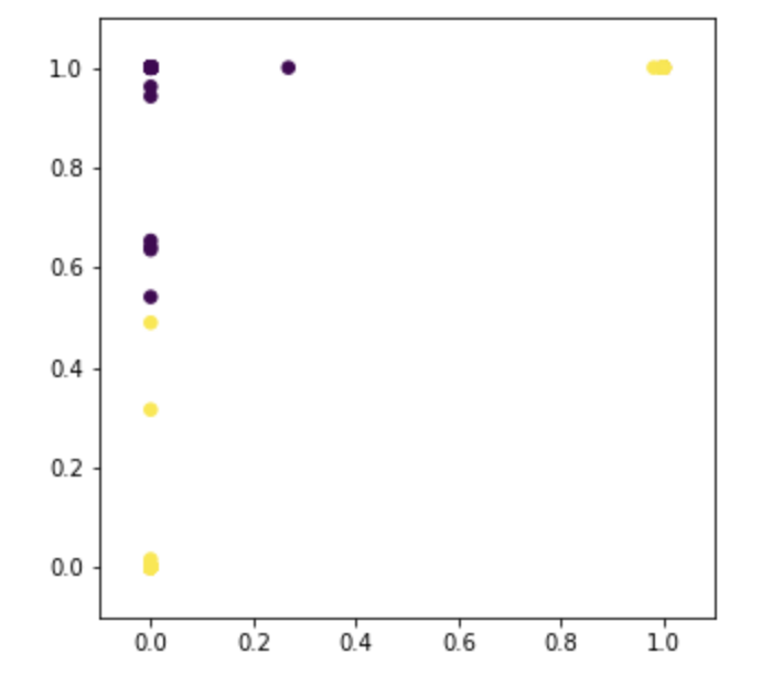

Now, how are the initial data transformed into these values? We can animate this process:

现在，如何将初始数据转换为这些值？ 我们可以对此过程进行动画处理：

• in the beginning, we have the original dataset (which is not, remember, linearly separable)
  一开始，我们有原始数据集(记住，这是线性可分离的)
• in the end, we have will have the transformed data in the (0,1) square because the sigmoid function has an output between 0 and 1. And do you see the form of the data? Yes, that’s when the magic happens…
  最后，我们将在(0,1)平方中拥有转换后的数据，因为Sigmoid函数的输出在0到1之间。您看到数据的形式了吗？ 是的，那就是魔术发生的时候……

输出神经元的性质 (Nature of the output neuron)

We can see that in the end, the dataset becomes linearly separable! For binary classification, the output neuron is a Logistic Regression. And it is easy to find a linear decision boundary. In this case, the hyperplane separator will be a straight line.

我们可以看到，最终，数据集变为线性可分离的！ 对于二进制分类，输出神经元是Logistic回归。 而且很容易找到线性决策边界。 在这种情况下，超平面分隔符将是一条直线。

So the intuition behind a neural network is that the hidden layers transform the non-linearly separable initial data into a space where they are almost linearly separable.

因此，神经网络背后的直觉是，隐藏层将非线性可分离的初始数据转换为几乎可以线性分离的空间。

神经网络的整体结构 (The whole structure of the neural network)

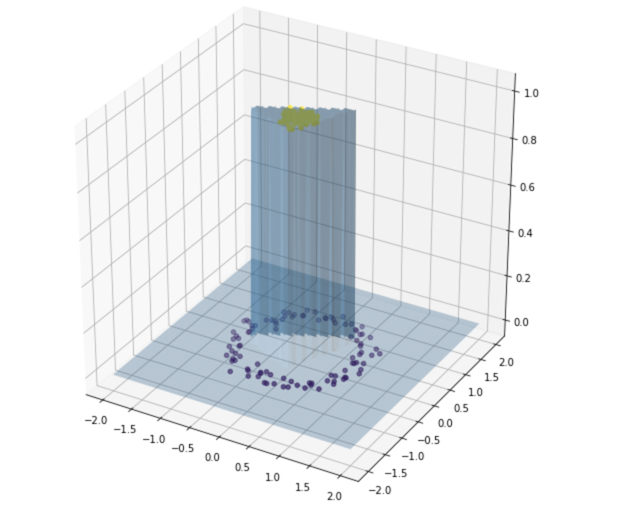
Combining the hidden layer and the output layer, we have a surface, and we can visualize it below. It is a surface because the input has 2 variables, and the output is the probability, so a number that we can represent by the z-axis.

将隐藏层和输出层结合起来，我们有了一个表面，我们可以在下面对其进行可视化。 它是一个曲面，因为输入有2个变量，而输出是概率，因此我们可以用z轴表示一个数字。

Now we can see that the two neurons “cut” the two frontiers between the two classes.

现在我们可以看到两个神经元“切开”了这两个类别之间的两个边界。

稍复杂的数据 (Slightly more complex data)

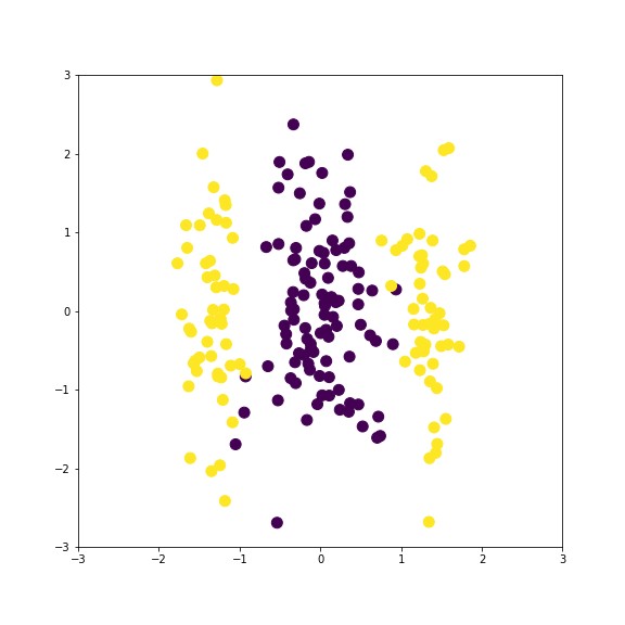
Now let consider the dataset below. One class is inside another with a circular form. Before using a Neural Network, which algorithms would solve this problem?

现在，让我们考虑下面的数据集。 一类以圆形形式存在于另一类内部。 在使用神经网络之前，哪种算法可以解决此问题？

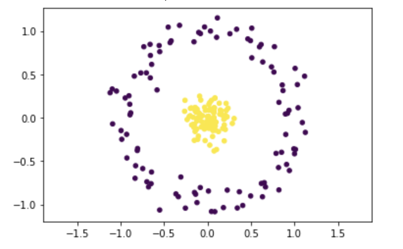
• Quadratic Discriminant Analysis is a suitable candidate, because the two classes have different covariance matrices with the same centers. The decision boundary will an almost perfect circle to separate the yellow dots from the purple points.

  二次判别分析是合适的候选方法，因为这两个类别具有相同中心的不同协方差矩阵。 决策边界将是一个几乎完美的圆圈，用于将黄色点与紫色点分开。

• SVM with an RBF (Radial Basis Function) kernel will also be perfect.

  具有RBF (径向基函数)内核的SVM也将是完美的。

• What about a Neural Network? Two neurons mean that you “cut” only twice, here we need at least three.

  神经网络呢？ 两个神经元意味着您只“切割”两次，这里我们至少需要三个。

最终神经网络表示 (Final Neural Network representation)

We can first see the final surface below and the decision boundary is actually a sort of triangle.

我们首先可以看到下面的最终曲面，而决策边界实际上是一种三角形。

隐藏层的转换 (Transformation of the hidden layer)

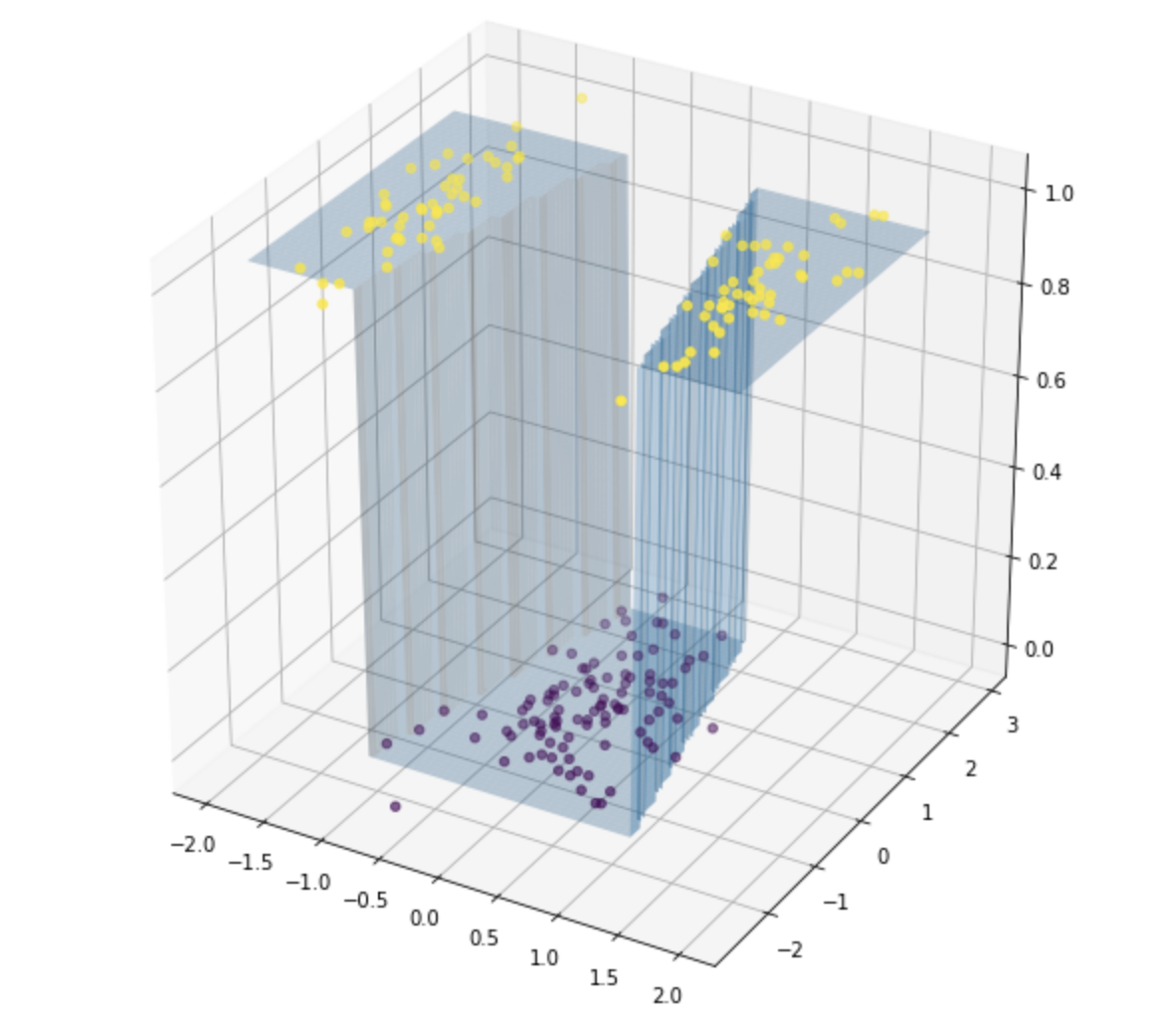
The initial 2D space is transformed into a 3D space, with 3 neurons. And we can animate this transformation.

最初的2D空间转换为具有3个神经元的3D空间。 我们可以为这种转换设置动画。

• In the beginning, the dataset is on a plane. We will consider that the value of the z-axis is zero.
  最初，数据集在平面上。 我们将认为z轴的值为零。
• In the end, the dataset is mapped into the (0,1) cube because the output of the sigmoid function is between 0 and 1.
  最后，由于Sigmoid函数的输出在0到1之间，因此数据集被映射到(0,1)多维数据集。

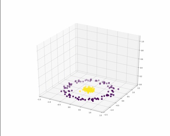
Now can you see that the dataset is almost linearly separable in this cube? Let’s create another animation by rotating the cube. Now you see that with a plane, we can easily separate the yellow dots from the purple ones?

现在，您可以看到该多维数据集中的数据集几乎是线性可分离的吗？ 让我们通过旋转立方体来创建另一个动画。 现在您看到了，使用飞机，我们可以轻松地将黄色点与紫色点分开吗？

In order to understand how algorithms work, I like to create visualizations with simple data. If you also find them helpful, please comment.

为了理解算法的工作原理，我喜欢用简单的数据创建可视化效果。 如果您还发现它们有帮助，请发表评论。

The plots are first created with python, then I use gifmaker to animate them.

这些图首先使用python创建，然后使用gifmaker对其进行动画处理。

翻译自: https://towardsdatascience.com/animations-of-neural-networks-transforming-data-42005e8fffd9

马斯克神经网络转换器