时间序列预测预测时间段_应用时间序列预测：美国住宅

最新推荐文章于 2024-09-15 22:31:42 发布

weixin_26746401

最新推荐文章于 2024-09-15 22:31:42 发布

阅读量487

点赞数

文章标签： python 机器学习 java 人工智能算法

原文链接：https://towardsdatascience.com/applied-time-series-forecasting-residential-housing-in-the-us-f8ab68e63f94

版权

本文探讨了如何使用时间序列预测方法对美国住宅市场进行预测，分析了预测时间段内的住宅房价趋势。

摘要由CSDN通过智能技术生成

时间序列预测预测时间段

1.简介 (1. Introduction)

During these COVID19 months housing sector is rebounding rapidly after a downtime since the early months of the year. New residential house construction was down to about 1 million in April. As of July 1.5 million new houses are under construction (for comparison, in July of 2019 it was 1.3 million). The Census Bureau report released on August 18 shows some pretty good indicators for the housing market.

自今年初以来，在经历了停工之后，在这19个COVID19个月中，住房行业Swift反弹。四月份的新住宅建设量降至约100万套。截至7月，正在建造150万套新房屋(相比之下，2019年7月为130万套)。人口普查局 8月18日发布的报告显示了一些相当好的房地产市场指标。

New house construction plays a significant role in the economy. Besides generating employment it simultaneously impacts timber, furniture and appliance markets. It’s also an important indicator of the overall health of the economy.

新房建设在经济中起着重要作用。除了创造就业机会，它同时影响木材，家具和家电市场。它也是经济整体健康状况的重要指标。

So one might ask, how will this crucial economic indicator play out the next few months and years to come after the COVID19 shock?

因此，有人可能会问，在COVID19冲击之后的几个月和几年中，这一至关重要的经济指标将如何发挥作用？

Answering these questions requires some forecasting.

回答这些问题需要一些预测。

The purpose of this article is to make short and medium-term forecasting of residential construction using a popular time series forecasting model called ARIMA.

本文的目的是使用流行的时间序列预测模型ARIMA对住宅建筑进行短期和中期预测。

Even if you are not much into the housing market but are interested in data science, this is a practical forecasting example that might help you understand how forecasting works and how to implement a model in real-world application cases.

即使您对房地产市场的兴趣不大，但对数据科学感兴趣，这也是一个实用的预测示例，可以帮助您了解预测的工作原理以及如何在实际应用案例中实现模型。

2.方法摘要 (2. Methods summary)

The objective is forecasting the construction of residential housing units in the short and medium-term using historical data obtained from census.gov database. Note that in the Census Bureau database, you’ll see there’re several datasets on housing indicators including “housing units started” and “housing units completed”; I’m using the latter for this article.

目的是使用从census.gov数据库获得的历史数据预测短期和中期的住宅单元建设。请注意，在人口普查局数据库中，您会看到有关房屋指标的多个数据集，包括“房屋单元已开始”和“房屋单元已完成”；我在本文中使用后者。

Census Bureau is a great source of time series data of all kinds on a large number of social, economic and business indicators. So if you are interested in time series analysis and modeling and want to avoid toy datasets, the Census Bureau is a great place to check out.

人口普查局是有关大量社会，经济和商业指标的各种时间序列数据的重要来源。因此，如果您对时间序列分析和建模感兴趣，并且希望避免使用玩具数据集，那么人口普查局是个很好的结帐地点。

I am doing the modeling in R programming environment. Python has great libraries for data science and machine learning modeling, but in my opinion, R has the best package, calledfpp2, developed by Rob J Hyndman, for time series forecasting.

我正在R编程环境中进行建模。 Python拥有用于数据科学和机器学习建模的出色库，但我认为R具有由Rob J Hyndman开发的用于时间序列预测的最佳软件包fpp2 。

There are many methods for time series forecasting, and I have written about them in a few articles before (you can check out this and this), but for this analysis I am going to use ARIMA. Before settling on ARIMA I ran a couple of other models — Holt-Winter and ETS — but found that ARIMA has a better performance for this particular dataset.

时间序列预测有很多方法，我之前已经在几篇文章中对此进行了介绍(您可以查看this和this )，但是对于此分析，我将使用ARIMA。在着手ARIMA之前，我还运行了其他几个模型(Holt-Winter和ETS)，但是发现ARIMA对于此特定数据集具有更好的性能。

3.数据准备 (3. Data preparation)

The only library I am using is fpp2. If you install this library all required dependencies will accompany.

我使用的唯一库是fpp2 。如果安装此库，则所有必需的依赖项都会伴随。

After importing data in the R programming environment (RStudio) I call the head() function.

在R编程环境(RStudio)中导入数据后，我调用head()函数。

# import library
library(fpp2)# import data
df = read.csv("../housecons.csv", skip=6)# check out first few rows
head(df)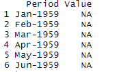

I noticed that the first few rows are empty, so I opened the CSV file outside of R to manually inspect for missing values and found that the first data did not appear until January of 1968. So I got rid of the missing values with a simple function na.omit().

我注意到前几行是空的，因此我在R之外打开了CSV文件以手动检查缺失值，发现直到1968年1月才出现第一个数据。因此，我用一个简单的方法消除了缺失值函数na.omit() 。

# remove missing values
df = na.omit(df)# check out the rows again
head(df)

As you notice in the dataframe above, it has two columns — time stamp and the corresponding values. You might think it is already a time series data so let’s go ahead and build the model. Not so fast, the dataframe may look like a time series but it’s not in a format that is compatible with the modeling package.

如您在上面的数据框中所注意到的，它具有两列-时间戳和相应的值。您可能会认为它已经是时间序列数据，所以让我们继续构建模型。数据帧的速度不是很快，可能看起来像一个时间序列，但格式与建模包不兼容。

So we need to do some data processing.

因此，我们需要进行一些数据处理。

As a side note, not just this dataset, any dataset you use for this kind of analysis in any package, you need to do pre-processing. This is an extra step but a necessary one. After all, this is not a cleaned, toy dataset that you typically find on the internet!

附带说明一下，您不仅需要此数据集，还需要对用于任何软件包中的此类分析的任何数据集进行预处理。这是一个额外的步骤，但却是必要的步骤。毕竟，这不是通常在互联网上找到的干净的玩具数据集！

# keep only `Value` column
df = df[, c(2)]# convert  values into a time series object
series = ts(df, start = 1968, frequency = 12)# now check out the series
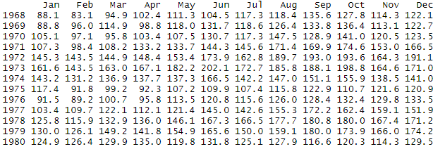
print(series)

The codes above are self-explanatory. Since we got rid of the “Period” column, I had to tell the program that the values start from 1968 and it’s an annual time series with 12-month frequency.

上面的代码是不言自明的。自从我们删除了“ Period”一栏之后，我不得不告诉程序该值始于1968年，它是一个12个月一次的年度时间序列。

The original data was in long-form, now after processing it is converted to a wide-form so you can now see a lot of data in a small window.

原始数据采用长格式，现在经过处理后将转换为宽格式，因此您现在可以在一个小窗口中看到大量数据。

We are now done with data processing. Was that easy to process data for time series compared to other machine learning algorithms? I bet it was.

现在，我们完成了数据处理。与其他机器学习算法相比，这样容易处理时间序列数据吗？我敢打赌

Now that we have the data that we needed, shall we go ahead and build the model?

现在我们有了所需的数据，我们是否应该继续构建模型？

Not so fast!

没那么快！

4.探索性分析 (4. Exploratory analysis)

Exploratory data analysis (EDA) may not seem like a pre-requisite, but in my opinion it is! And it’s for two reasons. First, without EDA you are absolutely blinded, you will have no idea what’s going into the model. You kind of need to know what raw material is going into the final product, don’t you?

探索性数据分析(EDA)似乎不是先决条件，但我认为是！这有两个原因。首先，如果没有EDA，您绝对是盲目的，您将不知道模型会发生什么。您有点需要知道最终产品将使用哪种原材料，不是吗？

The second reason is an important one. As you will see later, I had to test the model on two different input data series for model performance. I only did this extra step after I discovered that the time series is not smooth, it has a structural break, which influenced the model performance (check out the figure below, do you see the structural break?).

第二个原因很重要。稍后您将看到，我必须在两个不同的输入数据序列上测试模型的模型性能。我仅在发现时间序列不平滑，有结构性中断之后才执行此额外步骤，该结构性中断影响了模型性能(请查看下图，您看到结构性中断了吗？)。

Visualizing the series

可视化系列

The nice thing about the fpp2package is that you don’t have to separately install visualization libraries, it’s already built-in.

关于fpp2软件包的fpp2是您不必单独安装可视化库，它已经内置。

# plot the series
autoplot(series) + 
  xlab(" ") + 
  ylab("New residential construction '000") + 
  ggtitle(" New residential construction") + 
  theme(plot.title = element_text(size=8))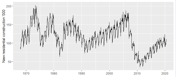

It’s just one single plot above, but there is so much going on. If you are a data scientist, you could stop here and take a closer look and find out how many bits of information you could extract from this figure.

这只是上面的一个图，但是发生了很多事情。如果您是一名数据科学家，则可以在这里停下来仔细观察，找出可以从该图中提取多少信息。

Here is my interpretation:

这是我的解释：

the data has a strong seasonality;
数据具有很强的季节性；
it also shows some cyclic behavior until c.1990, which then disappeared;
它也显示出一些周期性的行为，直到1990年左右才消失。
the series remained relatively stable since 1992 until the housing crisis;
自1992年以来，直到住房危机之前，该系列一直保持相对稳定；
the structural break due to market shock is clearly visible around 2008;
在2008年左右，市场冲击引起的结构性破坏显而易见。
the market is recovering since c. 2011 and growing steadily;
自c。开始市场复苏。 2011年并稳步增长；
2020 has yet another shock from COVID19. It’s not clearly visible in this figure, but if you zoom in you can detect it.
2020年又使COVID19感到震惊。在此图中看不到清晰可见的图像，但是如果放大可以检测到。

So much information you are able to extract from just a simple figure and these are all useful bits of information for building intuition before building models. That is why EDA is so essential in data science.

您可以从一个简单的图形中提取出如此多的信息，这些都是在构建模型之前建立直觉的有用信息。这就是为什么EDA在数据科学中如此重要的原因。

Trend

趋势

The overall trend in the series is already visible in the first figure, but if you want better visibility of the trend you can do that by removing seasonality.

该系列的总体趋势已经在第一个图中显示出来了，但是如果您想更好地了解趋势，可以通过消除季节性来实现。

# remove seasonality (monthly variation) to see yearly changesseries_ma = ma(series, 12)
autoplot(series_ma) + 
  xlab("Time") + ylab("New residential construction '000")+
  ggtitle("Series after removing seasonality" )+
  theme(plot.title = element_text(size=8))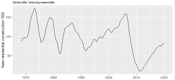

Seasonality

季节性

After seeing the general annual trend if you want to only focus on seasonality you could do that too with a seasonal sub-series plot.

在看到总体年度趋势之后，如果您只想关注季节性，则也可以使用季节性子系列图来实现。

# Seasonal sub-series plot 
series_season = window(series, start=c(1968,1), end=c(2020,7))
ggsubseriesplot(series_season) + 
  ylab(" ") +
  ggtitle("Seasonal subseries plot") +
  theme(plot.title = element_text(size=10))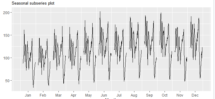

Time series decomposition

时间序列分解

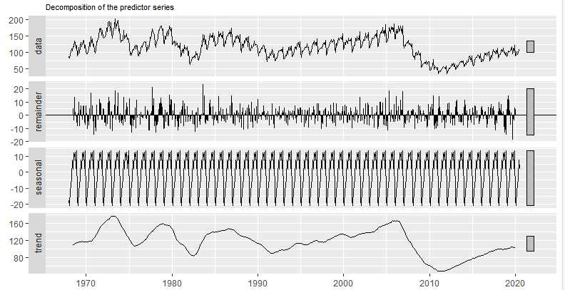
There is a nice way to show everything in one figure — it’s called the decomposition plot. Basically it is a composite of four information:

有一种很好的方法可以在一个图中显示所有内容-这称为分解图。基本上，它是四个信息的组合：

the original series (i.e. data)
原始系列(即数据)
trend
趋势
seasonality
季节性
random component
随机成分

# time series decomposition
autoplot(decompose(predictor_series)) + 
ggtitle("Decomposition of the predictor series")+
theme(plot.title = element_text(size=8))

The random data part is in this decomposition plot is the most interesting to me, since this component actually determines the uncertainty in forecasting. The smaller this random component the better.

这个分解图中的随机数据部分对我来说是最有趣的，因为此组件实际上确定了预测中的不确定性。该随机分量越小越好。

Zooming in

放大

We could also zoom in on a specific part of the data series. For example, below I zoomed in to see the good times (1995–2005) and bad times (2006–2016) in the housing market.

我们还可以放大数据系列的特定部分。例如，下面我放大查看房地产市场的好时光(1995-2005)和不好的时光(2006-2016)。

# zooming in on high time
series_downtime = window(series, start=c(1993,1), end=c(2005,12))
autoplot(series_downtime) + 
  xlab("Time") + ylab("New residential construction '000")+
  ggtitle(" New residential construction high time")+
  theme(plot.title = element_text(size=8))# zooming in on down time
series_downtime = window(series, start=c(2005,1), end=c(2015,12))
autoplot(series_downtime) + 
  xlab("Time") + ylab("New residential construction '000")+
  ggtitle(" New residential construction down time")+
  theme(plot.title = element_text(size=8))

Enough of exploratory analysis, now let’s move on to the fun part of model building, shall we?

足够的探索性分析之后，现在让我们继续进行模型构建的有趣部分，对吧？

5. ARIMA的预测 (5. Forecasting with ARIMA)

I already mentioned the rationale behind choosing ARIMA for this forecasting and it is because I tested the data with two other models but ARIMA showed a better performance.

我已经提到选择ARIMA进行此预测的基本原理，这是因为我用其他两个模型测试了数据，但是ARIMA显示出更好的性能。

Once you have your data preprocessed and ready to use, building the actual model is surprisingly easy. As an aside, it is also the case in most modeling exercise; writing codes and executing models is a small part of the whole process you need to go through — from data gathering & cleaning, to building intuition to finding the right model.

一旦对数据进行了预处理并可以使用，构建实际模型就非常简单。顺便说一句，在大多数建模练习中也是如此。编写代码和执行模型只是您需要经历的整个过程的一小部分-从数据收集和清理到建立直觉到找到正确的模型。

I followed 5 simple steps for implementing ARIMA:

我遵循了5个简单的步骤来实现ARIMA：

1 ) determining the predictors series

1)确定预测变量序列

2 ) model parameterization

2)模型参数化

3 ) plotting forecast values

3)绘制预测值

4 ) making a point forecast for a specific year

4)预测特定年份的分数

5 ) model evaluation/accuracy test

5)模型评估/准确性测试

Below you get all the codes needed for model implementation.

在下面，您可以获得模型实现所需的所有代码。

# determine the predictor series (in case you choose a subset of the series)
predictor_series = window(series, start=c(2011,1), end=c(2020,7))
autoplot(predictor_series) + labs(caption = " ")+ xlab("Time") + ylab("New residential construction '000")+
  ggtitle(" Predictor series")+
  theme(plot.title = element_text(size=8))# decomposition
 options(repr.plot.width = 6, repr.plot.height = 3)
 autoplot(decompose(predictor_series)) + ggtitle("Decomposition of the predictor series")+
 theme(plot.title = element_text(size=8))# model
forecast_arima = auto.arima(predictor_series, seasonal=TRUE, stepwise = FALSE, approximation = FALSE) 
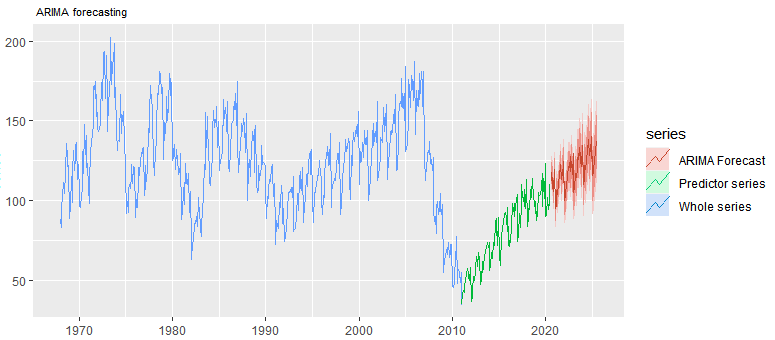
forecast_arima = forecast(forecast_arima, h=60)# plot
autoplot(series, series=" Whole series") +
  autolayer(predictor_series, series=" Predictor series") +
  autolayer(forecast_arima, series=" ARIMA Forecast") +
  ggtitle(" ARIMA forecasting") +
  theme(plot.title = element_text(size=8))# point forecast
point_forecast_arima=tail(forecast_arima$mean, n=12)
point_forecast_arima = sum(point_forecast_arima)
cat("Forecast value ('000): ", round(point_forecast_arima))print('')
cat(" Current value ('000): ", sum(tail(predictor_series, n=12))) # current value# model description
forecast_arima['model']# accuracy
accuracy(forecast_arima)

Like I said before, I ran ARIMA with two different data series, the first one was the whole data series from 1968 to 2020. As you see below, the forecasted values are kind of flat (red series) and come with a lot of uncertainties.

就像我之前说过的那样，我使用两个不同的数据系列运行ARIMA，第一个是1968年至2020年的整个数据系列。正如您在下面看到的那样，预测值有点平坦(红色系列)，并且存在很多不确定性。

The forecast looked a bit unrealistic to me given the trend over the last 10 years. You might think it is due to COVID19 impact? I don’t think so, because the model shouldn’t have picked up that signal just yet since COVID impact is a tiny part of the whole series.

考虑到过去10年的趋势，这一预测对我而言似乎有些不切实际。您可能会认为是由于COVID19的影响？我不这么认为，因为COVID的影响只是整个系列的一小部分，因此该模型还不应该接收该信号。

Then I realized that this uncertainty is because of the historical features in the series, including the uneven cycles and trend and the structural break. So I made the decision to use the last 10 years data as a predictor.

然后我意识到这种不确定性是由于该系列的历史特征，包括周期和趋势的不均匀以及结构性断裂。因此，我决定使用最近10年的数据作为预测指标。

The figure below is how it looks like once we use a subset of the series as a predictor. You can just visually compare the forecast area and the associated uncertainties (in red) between the two figures.

下图是一旦我们使用系列的子集作为预测变量后的样子。您可以直观地比较两个数字之间的预测区域和相关的不确定性(红色)。

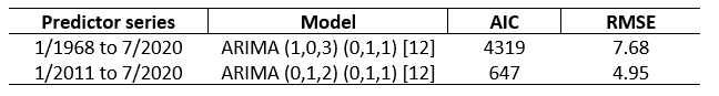
Below is more a quantitative way of comparing the performance of two models based on two input series. As you can see both the AIC and RMSE have dramatically declined to give the second model a solid performance.

下面是一种比较定量的方法，用于比较基于两个输入序列的两个模型的性能。如您所见，AIC和RMSE都大大降低了第二模型的性能。

预测值 (Forecast values)

Enough about the model building process, but this article is about doing an actual forecast with a real-world dataset. Below are the forecast values for new residential house construction in the United States.

关于模型构建的过程已经足够了，但是本文是关于使用真实数据集进行实际预测的。以下是美国新住宅建筑的预测值。

Current value (‘000 units): 1248
当前值('000单位)：1248
1-year forecast (‘000 units): 1310
1年预测(000个单位)：1310
5-year forecast (‘000 units): 1558
五年预测('000单位)：1558

6。结论 (6. Conclusions)

If the residential house construction continues along with the trend, 300K new residential housing units are expected to be built over the next 5 years. But this needs to be closely watched as the impact of COVID19 shock might be more apparent in the next few months.

如果住宅建设继续保持这种趋势，那么未来5年预计将建造30万套新住宅。但这需要密切注意，因为在接下来的几个月中，COVID19冲击的影响可能会更加明显。

I probably could’ve gotten a better model by tuning parameters or finding another model, but I wanted to keep it simple. In fact, as the adage goes, all models are wrong but some are useful. Hopefully, this AIMA model was useful in understanding some market dynamics.

我可能可以通过调整参数或找到其他模型来获得更好的模型，但我想保持简单。实际上，正如谚语所说，所有模型都是错误的，但有些模型是有用的。希望该AIMA模型有助于理解某些市场动态。