如何进行数据分析统计_对您不了解的数据集进行统计分析

如何进行数据分析统计

Recently, I took the opportunity to work on a competition held by Wells Fargo (Mindsumo). The dataset provided was just a bunch of numbers in various columns with no indication of what the data might be. I always thought that the analysis of data required some knowledge and understanding of the data and the domain to perform an efficient analysis. I have attached a sample below. It consisted of columns from X0 to X29 which consisted of continuous values and XC which consisted of categorical data i.e. 30 variables in total. I set out on further analysis on the entire dataset to understand the data.

[R ecently，我趁机工作由举办的比赛富国银行(Mindsumo) 。 提供的数据集只是各个列中的一堆数字，没有指示数据可能是什么。 我一直认为，数据分析需要对数据和领域有一定的了解和理解，才能进行有效的分析。 我在下面附上了一个样本。 它由从X0到X29的列组成，这些列由连续值组成，而XC则由分类数据组成，即总共30个变量。 我着手对整个数据集进行进一步分析以了解数据。

连续变量的正态性检查 (Normality check of continuous variables)

I used the QQ plot to determine the normality distribution of the variables and understand if there is any skew in the data. All the data points were normally distributed with very less deviation which required no processing of the data to be done at this point to attain a Gaussian distribution. I prefer a QQ plot for the initial analysis because it makes it very easy to analyze the data and determine the type of distribution be it Gaussian distribution, uniform distribution, etc.

我使用QQ图来确定变量的正态分布，并了解数据中是否存在任何偏差。 所有数据点均以极小的偏差进行正态分布，因此在这一点上无需对数据进行任何处理即可获得高斯分布。 我更喜欢使用QQ图进行初始分析，因为它使分析数据和确定分布类型变得非常容易，包括高斯分布，均匀分布等。

Once the data is determined to be a normal distribution using the QQ plot, a Shapiro Wilk test can be performed to confirm the hypothesis. It has been deigned specifically for normal distributions. The null hypothesis, in this case, is that the variable is normally distributed. If the p value obtained is less than 0.05 then the null hypothesis is rejected and it is assumed that the variable is not normally distributed. All the values seem to be greater than 0.5 which means that all the variables follow a normal distribution.

一旦使用QQ图确定数据为正态分布，就可以执行Shapiro Wilk检验来确认假设。 专为正态分布而设计。 在这种情况下，零假设是变量是正态分布的。 如果获得的p值小于0.05，则拒绝零假设，并假设变量不是正态分布的。 所有值似乎都大于0.5，这意味着所有变量都遵循正态分布。

分类变量 (Categorical variable)

I checked the distribution of the categorical variable to check if the points in the dataset were equally distributed. The distribution of the variables was as shown below. The variable consisted of 5 unique values (A,B,C,D and E) with all the values being more or less equally distributed.

我检查了分类变量的分布，以检查数据集中的点是否均匀分布。 变量的分布如下所示。 该变量由5个唯一值(A，B，C，D和E)组成，所有值或多或少均等地分布。

I used a One-Hot Encoding mechanism to convert the categorical variables to a binary variable for each resulting categorical value as shown below. Although this resulted in an increase in dimensionality, I was hoping to check for correlations later on and remove or merge certain rows.

我使用单点编码机制将每个结果分类值的分类变量转换为二进制变量，如下所示。 尽管这导致维数增加，但我希望以后再检查相关性，并删除或合并某些行。

数据关联 (Data Correlation)

Correlation is an important technique which helps in determining the relationships between the variables and weeding out highly correlated data. The reason we do this because we don't want variables that are highly correlated with each other since they affect the final dependent variable in the same way. The correlation values range from -1 to 1 with a value of 1 signifying a strong, positive correlation between the two and a value of -1 signifying a strong, negative correlation. We also calculate the statistical significance of the correlations to determine if the null hypothesis (There is no correlation) is valid or not. I have taken three values as benchmarks for measuring statistical significance — 0.1, 0.05 and 0.01. The below table is a small sub sample of the correlation values for each set of variables. A p value which is less than 0.01 signifies a high statistical significance and that the null hypothesis can be rejected which is represented by 3 ‘*’ while the statistical significance is lesser if the p-value is lesser than 0.1 but greater than 0.05 which is represented by 1 ‘*’.

关联是一项重要的技术，可帮助确定变量之间的关系并清除高度相关的数据。 我们之所以这样做，是因为我们不希望变量之间具有高度相关性，因为它们以相同的方式影响最终的因变量。 相关值的范围是-1到1，值1表示两者之间的强正相关，值-1表示强的负相关。 我们还计算了相关性的统计显着性，以确定零假设(无相关性)是否有效。 我已经采取三个值作为基准，用于测量统计显着性- 0.1，0.05和0.01。 下表是每组变量的相关值的一小部分子样本。 如果p值小于0.01，则表示具有较高的统计显着性，并且可以拒绝由3 '*'表示的原假设，而如果p值小于0.1但大于0.05，则统计学显着性较小。用1' *'表示 。

The dataset above did not have any values which had a high correlation value. Thus, I safely went ahead with the assumption that the values were not related to each other. I further explored the correlation of the variables with the dependent variable y.

上面的数据集没有任何具有高相关值的值。 因此，我可以安全地继续进行以下假设：这些值彼此无关。 我进一步探讨了变量与因变量y的相关性。

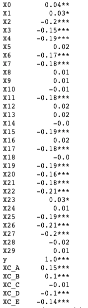
We are concerned with the prediction of the variable y. As seen, there are a lot of variables which don't have any correlation to y as well as are not statistically significant at all which means that the relationship is weak and we can safely exclude them from the final dataset. These include variables such as X5, X8, X9, X10, XC_C, etc. I have not excluded the other variables which have low correlation but high statistical significance as there may be a small sample which affects the final dependent variable and we cannot exclude them completely. We can further reduce the variables by merging some of them. We do this on the basis of variables which have the same correlation value with the y variable. These include —

我们关注变量y的预测。 可以看出，有很多变量与y没有任何关系，并且在统计上根本不重要，这意味着该关系很弱，我们可以安全地将它们从最终数据集中排除。 这些变量包括X5 ， X8 ， X9 ， X10 ， XC_C等。我没有排除其他相关性较低但具有统计学意义的变量，因为可能会有一个小的样本影响最终因变量，因此我们不能排除它们完全。 我们可以通过合并其中的一些变量来进一步减少变量。 我们基于与y变量具有相同相关值的变量进行此操作。 这些包括 -

• X7, X11, X17 and X21

  X7 ， X11 ， X17和X21

• X1 and X23

  X1和X23

• X22 and X26

  X22和X26

• X4, X15, X19 and X25

  X4 ， X15 ， X19和X25

I merged these variables using an optimization technique. Let us consider the variable, X1 and X23. I achieved this by assuming a linear relation mX1 + nX23 with y. For determining the maximum correlation, we have to calculate the optimum value for m and n. In all the cases, I assumed n to be 1 and solved for m. The equation is as shown below.

我使用优化技术合并了这些变量。 让我们考虑变量X1和X23 。 我通过假设线性关系m X1 + n X23与y来实现这一点。 为了确定最大相关性，我们必须计算m和n的最佳值。 在所有情况下，我都假定n为1并求解m。 公式如下所示。

Once n is set as 1, we can easily solve for m. This can be substituted in the above linear equation for each value. In this way, we can merge all the above variables. If the denominator is 0, m can be taken as 1 and the equation can be solved for n. Make sure that the correlation values are equal for both the variables. After merging, I generated the correlation table again.

将n设置为1后 ，我们可以轻松求解m。 可以在上面的线性方程式中将其替换为每个值。 这样，我们可以合并所有上述变量。 如果分母为0 ，则m可以取为1，并且该方程可以求解n 。 确保两个变量的相关值相等。 合并后，我再次生成了相关表。

We can see that the correlation values for the merged variables have increased and the statistical significance is high for all of them. I managed to reduce the number of variables from 30 to 15. I can now use these variables to feed it into my machine learning model and check the accuracy against the validation dataset.

我们可以看到，合并变量的相关值已经增加，并且所有变量的统计意义都很高。 我设法将变量的数量从30个减少到15个 。 现在，我可以使用这些变量将其输入到我的机器学习模型中，并根据验证数据集检查准确性。

训练和验证数据 (Training and Validating the data)

I chose a Logistic Regression model for the training and predicting on this dataset for multiple reasons —

由于多种原因，我选择了Logistic回归模型来对该数据集进行训练和预测-

• The dependent variable is binary
  因变量是二进制
• The independent variables are related to the dependent variable
  自变量与因变量有关

After training the model, I checked the model against the validation dataset and these are the results.

训练模型后，我对照验证数据集检查了模型，这些是结果。

The model had an accuracy of 99.6% with a F1 score of 99.45%.

该模型的accuracy为99.6％ ， F1 score为99.45％ 。

结论 (Conclusion)

This was a basic exploratory and statistical analysis to reduce the number of features and assure that there are no correlated variables in the final dataset. Using a few simple techniques, we can be assured of getting good results even if we do not understand what the data is initially. The main steps include ensuring a normal distribution of data and an efficient encoding scheme for the categorical variables. Further, the variables can be removed and merged based on correlation among them after which an appropriate model can be chosen for analysis. You can find the code repository at https://github.com/Raul9595/AnonyData.

这是一项基本的探索性和统计分析，目的是减少特征数量并确保最终数据集中不存在相关变量。 使用一些简单的技术，即使我们不了解最初的数据是什么，也可以确保获得良好的结果。 主要步骤包括确保数据的正态分布和有效的分类变量编码方案。 此外，可以基于变量之间的相关性来删除和合并变量，之后可以选择适当的模型进行分析。 您可以在https://github.com/Raul9595/AnonyData中找到代码存储库。

翻译自: https://towardsdatascience.com/statistical-analysis-on-a-dataset-you-dont-understand-f382f43c8fa5

如何进行数据分析统计