vlookup match_INDEX-MATCH — VLOOKUP功能的升级

最新推荐文章于 2024-10-02 10:53:34 发布

weixin_26746401

最新推荐文章于 2024-10-02 10:53:34 发布

阅读量363

点赞数

文章标签： python java

原文链接：https://towardsdatascience.com/index-match-an-upgrade-on-vlookup-functions-320e43253d15

版权

vlookup match

电子表格/索引匹配 (SPREADSHEETS / INDEX-MATCH)

In a previous article, we discussed about how and when to use VLOOKUP functions and what are the issues that we might face while using them. This article, on the other hand, will take you to a journey to understand an upgraded version of VLOOKUP. This upgrade is a combination of two functions in spreadsheets — INDEX and MATCH. Let us try and understand the working of INDEX-MATCH through the following example.

在上一篇文章中，我们讨论了如何以及何时使用VLOOKUP函数，以及在使用它们时可能遇到的问题。另一方面，本文将带您了解VLOOKUP的升级版本 。此升级是电子表格中两个功能的组合INDEX和MATCH 。让我们尝试通过以下示例来理解INDEX-MATCH的工作。

了解数据 (Understanding the Data)

As always, let us take an example from our favorite data source — Kaggle. The following screenshot is a small subset of the Netflix data which consists of TV shows and movies available on Netflix as of 2019.

与往常一样，让我们以我们最喜欢的数据源Kaggle为例。以下屏幕截图是Netflix数据的一小部分，其中包括截至2019年Netflix上可用的电视节目和电影。

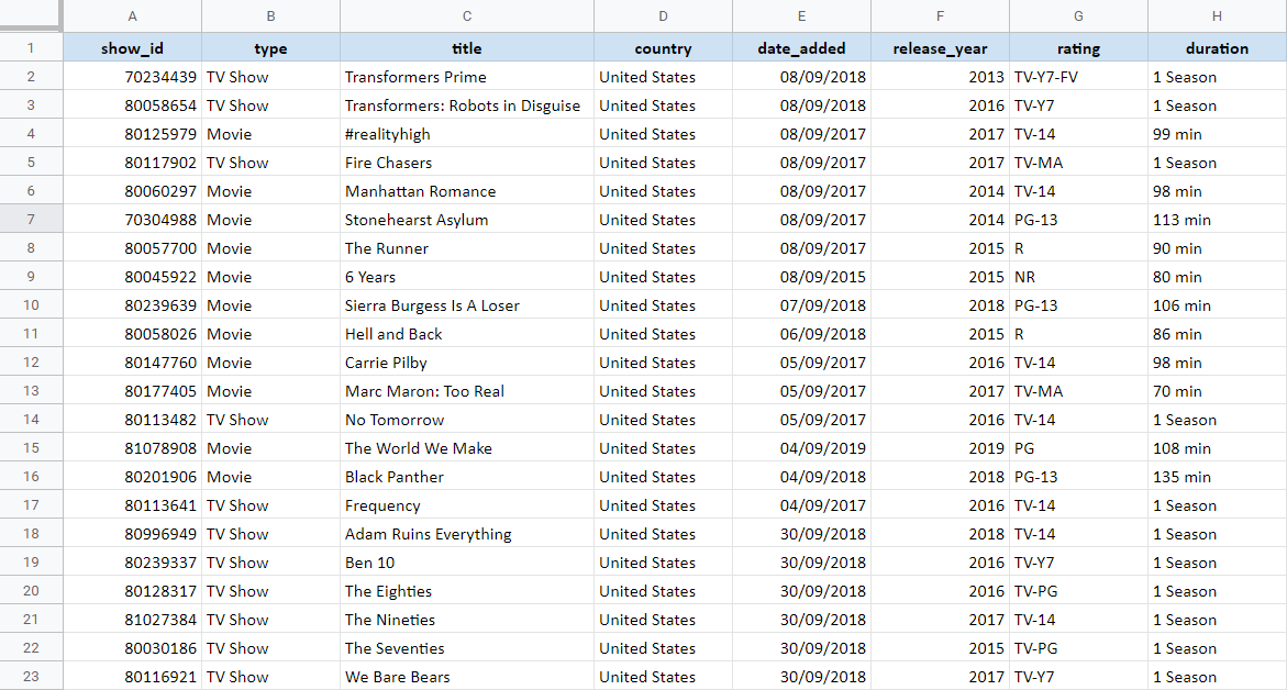
Image for post — Netflix Data for INDEX-MATCH demonstration

This dataset consists of different shows and movies along with their unique show_id, country we are considering, date when the show was added and the year when the entity was released. It also contains rating of the show/movie, duration and title of the content piece.

该数据集包含不同的节目和电影，以及它们唯一的show_id ，我们正在考虑的country ，添加节目的date和发布实体的year 。它还包含内容的放映/电影rating ， duration和title 。

Consider now that we want to create a search method where the user can select a title and we display information to the user regarding that title. This search method would look something like this:

现在考虑，我们想创建一种搜索方法，用户可以在其中选择title然后向用户显示有关该标题的信息。此搜索方法如下所示：

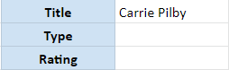
The user can input any title in the above example and we will try and find the type and rating of the title mentioned from the database. One of the simpler solutions to this is through VLOOKUP. We can easily find the rating of the title through it. Although, we would need to change the structure of the table to get the type of the title since VLOOKUP can only look to the right of the search value. Let’s see how can INDEX and MATCH formulas help us in solving this problem.

用户可以在上面的示例中输入任何title ，我们将尝试从数据库中查找提到的标题的type和rating 。一种更简单的解决方案是通过VLOOKUP。我们可以通过它轻松找到标题的等级。虽然，我们将需要更改表的结构以获取标题的类型，因为VLOOKUP 只能在搜索值的右侧查找。让我们看看INDEX和MATCH公式如何帮助我们解决此问题。

什么是索引？ (What is INDEX?)

INDEX formula in spreadsheets look something like this:

电子表格中的INDEX公式如下所示：

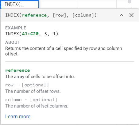
INDEX helps us in finding the content of the cell. It takes 3 inputs.

INDEX帮助我们找到单元格的内容。它需要3个输入。

Row: The number of rows from the beginning of the reference table where the value lies. This is an optional value. If no value is supplied, it will take the first row as the value.
行：从值所在的引用表的开头开始的行数。这是一个可选值。如果未提供任何值，则它将第一行作为值。
Column: The number of columns from the beginning of the reference table where the value lies. This is an optional value. If no value is supplied, it will take the first column as the value.
列：从值所在的参考表开始的列数。这是一个可选值。如果未提供任何值，则它将第一列作为值。

To find the type of the title ‘Carrie Pilby’ in our table, we apply the following formula:

要在我们的表格中找到标题“ Carrie Pilby”的类型，我们使用以下公式：

=INDEX(A1:H23,12,2)

We select the complete table as reference, we find that this movie title is in the 12th row and we know that the type of the title is stored in 2nd column of the reference table. This will give the result as ‘Movie’ which is absolutely correct!

我们选择完整的表作为参考 ，我们发现该电影标题位于第12行，并且知道标题的类型存储在参考表的第二列中。这将给出绝对正确的“电影”结果！

But did you notice any problems with this? We actually had to count the row number and the column number to get 12 and 2 as the parameters in the formula. This isn’t easy, is it? Let’s find out if there is any other way in the world which can help us in easing this process.

但是您注意到这个有什么问题吗？实际上，我们必须对行号和列号进行计数，以获得12和2作为公式中的参数。这不容易，是吗？让我们找出世界上是否还有其他方法可以帮助我们简化这一过程。

什么是MATCH？ (What is MATCH?)

MATCH formula in spreadsheets look something like this:

电子表格中的MATCH公式如下所示：

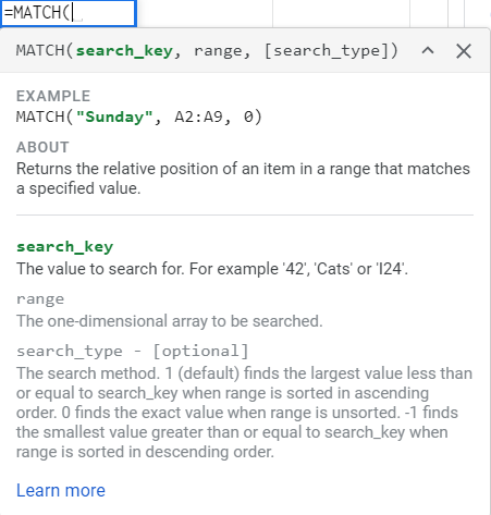
MATCH helps us in finding the relative position of the content in our table. It takes 3 inputs.

MATCH帮助我们找到表中内容的相对位置。它需要3个输入。

Search Key: The value that we want to find.
搜索键 ：我们要查找的值。
Range: The row/column in which the value is situated. Note that range can only take a row or a column, but not both.
范围：值所在的行/列。请注意，范围只能包含一行或一列，但不能同时包含两者。
Search Type: For all practical purpose, we set this value as zero. This indicates that we are finding the exact value. This is an optional term which takes the value as 1 by default.
搜索类型 ：出于所有实际目的， 我们将此值设置为零 。这表明我们正在寻找确切的值。这是一个可选术语，默认情况下将值设为1。

MATCH essentially gives us the row number or the column number of where the search term lies. Isn’t this the missing part of the INDEX puzzle we encountered earlier? We needed an easier way to find the row and column number of the search item, rather than counting it manually. And MATCH gives you exactly that!

MATCH本质上为我们提供了搜索词所在的行号或列号。这不是我们之前遇到的INDEX难题的缺失部分吗？我们需要一种更简单的方法来查找搜索项的行号和列号，而不是手动对其进行计数。而MATCH正是为您提供！

神圣的INDEX-MATCH婚姻 (The holy INDEX-MATCH matrimony)

The above explanation now allows us to join the INDEX and MATCH formulas together and get the information we require with the minimum amount of hassle. Here is how a general INDEX-MATCH formula would look like:

上面的解释现在使我们可以将INDEX和MATCH公式结合在一起，并以最少的麻烦获得所需的信息。通用INDEX-MATCH公式如下所示：

=INDEX(reference, MATCH(search_key, row, 0), MATCH(search_key, column, 0))

In the above formula, we provide a reference table to the INDEX, which is basically the data table where all the information is. Next, the first MATCH formula provides the row index of the search term and the second MATCH provides the column index of the search term. Finally, the combination of these two will provide the row and column index to the INDEX formula and we’ll get our desired result! Let’s try it out in our Netflix example.

在上面的公式中，我们提供了INDEX的参考表 ，它基本上是所有信息所在的数据表。接下来，第一个MATCH公式提供搜索项的行索引， 第二个 MATCH公式提供搜索项的列索引 。最后，这两者的结合将为INDEX公式提供行索引和列索引，我们将获得理想的结果！让我们在Netflix示例中尝试一下。

The above formula selects the entire table in first parameter of INDEX. Then it searches for the movie title mentioned in K1 through MATCH formula in the entire row of content titles, which is C1:C23. This will return whatever row number the title ‘Carrie Pilby’ is in. In the second MATCH, it searches for J2, which is the parameter that we want to find, in this case Type. This will return whatever column the column name ‘Type’ is in. And together it will provide the correct result i.e. Movie.

上面的公式在INDEX的第一个参数中选择整个表。然后，它通过MATCH公式在整个内容标题行(即C1：C23)中搜索K1中提到的电影标题。这将返回标题为“ Carrie Pilby”所在的行号。在第二个MATCH中，它将搜索J2，这是我们要查找的参数，在本例中为Type。这将返回列名“ Type”所在的任何列。并且一起提供正确的结果，即Movie。

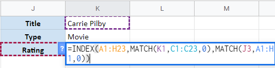
Similarly, here is the formula for how to match rating in the table for the given content title.

同样，这是有关如何匹配表中给定内容标题的评级的公式。

与VLOOKUP比较 (Comparing with VLOOKUP)

Often there will be comparisons on which formula to use to find the values of a given content. Although VLOOKUP is simpler to understand and provides an easy application, the INDEX-MATCH combination is a powerful match which provides the following advantages:

通常会比较使用哪个公式来查找给定内容的值。尽管VLOOKUP易于理解并且易于使用，但INDEX-MATCH组合是功能强大的匹配项，具有以下优点：

You can use INDEX-MATCH to find a value against multiple criteria. In the above examples, we found Type and Rating with content name criteria and parameter criteria. This wouldn’t have been easy to achieve in VLOOKUP.
您可以使用INDEX-MATCH 根据多个条件查找值 。在以上示例中，我们找到了带有内容名称标准和参数标准的Type和Rating 。这在VLOOKUP中并非容易实现。
VLOOKUP finds a match on the left and returns any value to the right of the search item. On the other hand, INDEX-MATCH can look both ways. In the above example, type was on the left of title and rating on the right, still it managed to find both the results correctly.
VLOOKUP在左侧找到一个匹配项，并在搜索项的右侧返回任何值。另一方面， INDEX-MATCH可以双向查看 。在上面的示例中，类型位于标题的左侧，评级位于右侧，但仍设法正确找到了两个结果。

Understanding INDEX-MATCH adds an extremely versatile tool in your spreadsheet armory. INDEX-MATCH along with the knowledge of Pivot Tables can really help you to improve your analytical skills. Let me know in comments if this was a helpful piece of content!

了解INDEX-MATCH可以在电子表格库中添加一个极其通用的工具。 INDEX-MATCH以及数据透视表的知识可以真正帮助您提高分析技能。在评论中让我知道这是否是有用的内容！