ggplot2简单使用_用ggplot2预测足球比分

ggplot2简单使用

胡闹 (Horsing Around)

In one of my earlier posts, I mentioned that the scores in a football match can be approximated somewhat using the Poisson distribution, but I didn’t go too much into the topic. Well, you’re in luck today… we’re going to have a look at the subject, and by the end of this post we’ll have Ggplot2 visual illustrating the likely scores of a football match, which really is excellent.

在我以前的一篇文章中，我提到足球比赛的得分可以使用泊松分布 ( Poisson distribution)进行某种程度的近似，但是我并没有过多地讨论这个话题。 好吧，今天您很幸运……我们将对这个话题进行一番探讨，在本博文结尾处，我们将使用Ggplot2视觉效果来说明足球比赛的可能得分，这确实很棒。

First off, a little bit on the roots of the Poisson distribution. The discovery of this probability distribution is attributed to Siméon Denis Poisson, a French mathematician from the nineteenth century. Like many of his contemporaries at the time, he dealt mainly with its theories. It wasn’t until Russian statistician Ladislaus Bortkiewicz published his book The Law of Small Numbers in 1898 that the Poisson distribution became widely used in practice.

首先，介绍一下泊松分布的根源。 这种概率分布的发现归因于19世纪法国数学家SiméonDenis Poisson 。 像当时的许多同时代人一样，他主要研究其理论。 直到俄国统计学家Ladislaus Bortkiewicz于1898年出版他的《 小数 定律》时，泊松分布才在实践中得到广泛使用。

Bortkiewicz famously had access to a data set of the Prussian army over a period of 20 years which recorded the number of soldiers that were killed by their horses’ kicks. Grim.

著名的Bortkiewicz可以使用20年来的普鲁士军队数据集，该数据集记录了被他们的马踢杀死的士兵人数。 严峻。

Anyway, he showed that these deaths could be approximated by the Poisson distribution, and the rest, as they say, is history.

无论如何，他证明了这些死亡可以通过泊松分布来估计，其余的，正如他们所说的，都是历史。

Now… how does one go from Prussian cavalry to football scores?

现在……从普鲁士骑兵到足球比分如何？

做我和你的屁股 (Making an Ass of U and Me)

Let’s first have a look at the basic assumptions that satisfy a Poisson process:

首先让我们看一下满足泊松过程的基本假设：

1. The probability of an event occurring in a given time interval does not vary with time

   在给定的时间间隔内发生事件的概率不会随时间变化

2. The events occur at random

   这些事件是随机发生的

3. The events occur independently

   事件独立发生

Now think of goals as an event in a football match. If we had a metric that could express a team’s scoring rate/intensity over 90 minutes, we can say that the first assumption is satisfied. This would’ve been a pain in the arse to define, but thankfully the sports nerds (people a hundred times more intelligent than me, I should add) have come up with expected goals (xG) for this. Thanks for today!

现在，将目标视为足球比赛中的一项活动。 如果我们有一个指标可以表示一支球队在90分钟内的得分率/强度，则可以说第一个假设已满足。 这本来很难定义，但是值得庆幸的是，那些运动狂的书呆子(我应该补充的人比我聪明一百倍)为此提出了预期的目标 (xG)。 感谢今天！

Next question- do goals occur randomly in a football match? That is to say, is there a particular point in time in a match when goals are more likely to be scored? This guy says no, and many other articles and studies also suggest that goals do occur at random in a football match. In practice, goals might not be as random as one might think but… we have enough evidence to argue that they are, so let’s tick that box and move on for now.

下一个问题-足球比赛中进球是否随机发生？ 也就是说，比赛中是否有特定的时间点更有可能进球？ 这个家伙说不，而且许多其他文章和研究还表明，足球比赛中确实会随机发生进球。 在实践中，目标可能不会像人们想象的那样随机，但是……我们有足够的证据证明它们是真实的，所以让我们在方框中打勾，然后继续。

Now for the final assumption- that being, goals are independent of one another. If a team is behind, surely the players are working harder to get back into the game to score an equaliser. Or perhaps if a team is already leading by 5 goals, the players might take their foot off the gas and let one in due to complacency. Either way, you have to say that goals don’t occur independently of one another, and using a basic Poisson process to model football scores starts to break down here.

现在，最后一个假设是，目标彼此独立。 如果有一支球队落后，那肯定是球员们正在更加努力地重新回到比赛中来得分。 或者，如果一支球队已经以5个进球领先，那么球员们可能会因为自满而放弃自己的力量而让一个人进入。 无论哪种方式，您都必须说目标不是彼此独立发生的，而使用基本的泊松过程来模拟足球得分的方法就此开始崩溃。

There are techniques to adjust for goal dependencies in a match, but we all have day jobs- so let’s leave that for another day… and agree for now that two out of three isn’t bad (also, I’m pushing to generate useful content innit, so here we are). For further reading, I suggest having a look at this fantastic blog post that has basically done a Bortkiewicz for football, showing you can approximate the number goals scored over a season with the Poisson distribution.

有一些技巧可以调整比赛中的目标依赖性，但我们都有日常工作，因此让我们再待一天……并且现在就同意，三分之二还不错(此外，我也在努力产生有用的信息)内容内容，所以我们在这里)。 为了进一步阅读，我建议您看一下这篇出色的博客文章 ，该文章基本上完成了Bortkiewicz的足球比赛，表明您可以使用泊松分布估算一个赛季的进球数。

蹄 (Hoof)

In my previous post on xG, I created a simple Poisson model to help predict the outcomes of a football match (home win, draw, away win) in R. We’re going to use something similar here, but focus more on obtaining the probabilities of the correct scores as an output.

在我以前关于xG的文章中，我创建了一个简单的Poisson模型来帮助预测R中的足球比赛(主场胜利，平局，客场胜利)的结果。我们将在此处使用类似的方法，但重点更多地放在获得正确分数的概率作为输出。

R has come a long way from its base heat map libraries which haven’t aged too well. Ggplot2 is a fantastic package which allows for all sorts of graphs and charts to be built. In order to use them, we have to first install some dependencies in RStudio:

R与尚未成熟的基础热图库相距很远。 Ggplot2是一个很棒的程序包，它允许构建各种图形和图表。 为了使用它们，我们必须首先在RStudio中安装一些依赖项：

install.packages('tidyr')
install.packages('dplyr')
install.packages('scales')
install.packages('ggplot2')library('tidyr')
library('dplyr')
library('scales')
library('ggplot2')

Cool, now let’s go back to one of our original assumptions- that teams have a constant scoring rate over 90 minutes in a football match. We’ll be using the shot-based xG taken from FiveThirtyEight’s model for the Champions League quarter-final between Barcelona and Bayern Munich (oh boy…). Let’s construct and source a ScoreGrid:

太酷了，现在让我们回到最初的假设之一：球队在一场足球比赛中90分钟内的得分均保持恒定。 我们将使用FiveThirtyEight模型中基于镜头的xG来进行巴塞罗那和拜仁慕尼黑之间的冠军联赛八强(哦，男孩……)。 让我们构造并获取一个ScoreGrid ：

ScoreGrid<-function(homeXg,awayXg){
  
  A <- as.numeric()
  B <- as.numeric()
  
  for(i in 0:9) {
    A[(i+1)] <- dpois(i,homeXg)
    B[(i+1)] <- dpois(i,awayXg)
  }
  
  A[11] <- 1 - sum(A[1:10])
  B[11] <- 1 - sum(B[1:10])
  
  name <- c("0","1","2","3","4","5","6","7","8","9","10+")
  zero <- mat.or.vec(11,1)
  
  C <- data.frame(row.names=name, "0"=zero, "1"=zero, "2"=zero, "3"=zero, "4"=zero,
                  "5"=zero, "6"=zero, "7"=zero,"8"=zero,"9"=zero,"10+"=zero)
  
  for(j in 1:11) {
    for(k in 1:11) {
      C[j,k] <- A[k]*B[j]
    }
  }
  
  colnames(C) <- name
  
  return(round(C*100,2)/100)
}

We’ve created a data frame with 11 columns and 11 rows, each entry representing a correct score. So the entry in [row i , column j] is going to be the score i,j with i being the home score and j as the away score. Hence entry [1,2] is going to be a 2–1 win for the away team. dpois helps to generate a random Poisson probability for each score i, given the homeXg and awayXg. Finally, we cap the individual scores at 9, and once we get to 10 we’re going to sum the probabilities together and group them as a single entry. It just makes things easier.

我们创建了一个包含11列11行的数据框，每个条目代表一个正确的分数。 因此，[ 第i行，第j列 ]中的条目将为得分i，j 和我在一起 是主场得分和j 作为客场得分。 因此，客队[ 1,2 ]将会是2-1的胜利。 给定homeXg和awayXg ， dpois有助于为每个分数i生成随机的泊松概率。 最后，我们将单个分数的上限设置为9，一旦达到10，我们将对这些概率求和，并将其分组为一个条目。 它只是使事情变得容易。

Let’s give it a quick spin. In the RStudio console, type

让我们快速旋转一下。 在RStudio控制台中，键入

ScoreGrid(1.7,1.1)

and you should get this:

你应该得到这个：

Football correct score grid. Image by author

足球正确比分网格。 图片作者

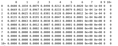
Nice grid, but not too easy on the eye.

漂亮的网格，但在眼睛上不太容易。

罗伯特·莱万戈阿尔斯基 (Robert Lewangoalski)

Let’s build the correct score visual now. We’re going to use geom_tile() in Ggplot2, which generates a nice heat map at the end. Here’s the code:

让我们现在构建正确的视觉分数。 我们将在Ggplot2中使用geom_tile() ，它最终会生成一个不错的热图。 这是代码：

ScoreHeatMap<-function(home,away,homeXg,awayXg,datasource){
  
  adjustedHome<-as.character(sub("_", " ", home))
  adjustedAway<-as.character(sub("_"," ",away))
  
  df<-ScoreGrid(homeXg,awayXg)
  
  df %>% 
    as_tibble(rownames = all_of(away)) %>%
    pivot_longer(cols = -all_of(away), 
                 names_to = home, 
                 values_to = "Probability") %>%
    mutate_at(vars(all_of(away), home), 
              ~forcats::fct_relevel(.x, "10+", after = 10)) %>% 
    ggplot() + 
    geom_tile(aes_string(x=all_of(away), y=home, fill = "Probability")) +   
    scale_fill_gradient2(mid="white", high = muted("red"))+
    theme(plot.margin = unit(c(1,1,1,1),"cm"),
          plot.title = element_text(size=20,hjust = 0.5,face="bold",vjust =4),
          plot.caption = element_text(hjust=1.1,size=10,face = "italic"), 
          plot.subtitle = element_text(size=12,hjust = 0.5,vjust=4),
          axis.title.x=element_text(size=14,vjust=-0.5,face="bold"),
          axis.title.y=element_text(size=14, vjust =0.5,face="bold"))+
    labs(x=adjustedAway,y=adjustedHome,
         caption=paste("xG Source:", datasource))+
    ggtitle(label = "Expected Scores", subtitle = paste(adjustedHome, "vs",adjustedAway,"xG:",homeXg,"-",awayXg))
  
}

Ggplot2 requires the input data to be a tidy dataframe, so the conversion from base R data.frame takes place on line 10 with pivot_longer. Next, we’ll need to convert all our vars to factors and sort the levels in the correct order (remember that 10+ is a factor, using as.numeric will just cause it to become an NA. We want it to be the final level in the list). This is done on line 14 with ~forcats::fct_relevel. Everything beyond that just contains the usual building blocks of a Ggplot2 graph.

Ggplot2要求输入数据是tidy数据帧，因此从基数R data.frame的转换发生在第10行的pivot_longer 。 接下来，我们需要将所有vars转换为factors并以正确的顺序对级别进行排序(请记住10+是因子，使用as.numeric只会使其变为NA 。我们希望它成为最终as.numeric列表中的级别)。 这是在第14行上使用~forcats::fct_relevel 。 除此之外的所有内容都包含Ggplot2图的通常构建块。

Right, here we go. Fire up the R console and enter the team names and xG inputs from wherever your source was from:

是的，我们开始。 启动R控制台，并从任何来源输入团队名称和xG输入：

ScoreHeatMap("Barcelona", "Bayern_Munich", 1.2, 5.6, "FiveThirtyEight")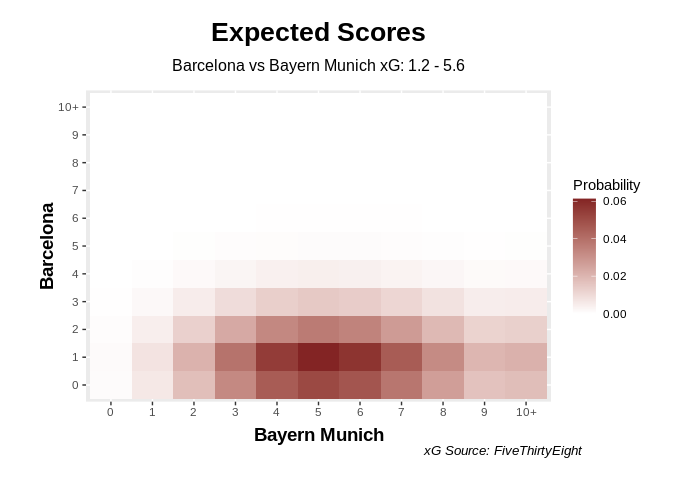

Barcelona vs Bayern Munich correct scores visualisation. Image by author

巴塞罗那vs拜仁慕尼黑正确的比分可视化。 图片作者

Men against boys in this match, and just by looking at the visualisation/heat map you can see the most likely score would have been 5–1 to Bayern Munich based on xG. In reality, Bayern actually won 8–2. Robert Lewangoalski indeed.

在这场比赛中男人对男孩的比赛，仅通过观察可视化/热图，您就可以得出基于xG的拜仁慕尼黑最可能的得分是5–1。 实际上，拜仁实际上赢了8-2。 Robert Lewangoalski的确如此。

One more to illustrate a closer match, yesterday evening’s Champions League final between Paris Saint-Germain and Bayern Munich:

昨天晚上巴黎圣日耳曼队和拜仁慕尼黑队之间的冠军联赛决赛还有另外一场比赛来说明一场更接近的比赛：

ScoreHeatMap("Paris_SG", "Bayern_Munich", 1.4,1.6,"FiveThirtyEight")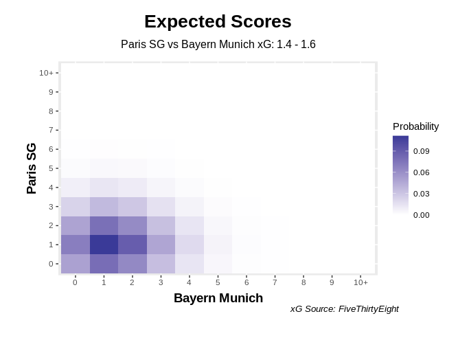

Paris Saint-Germain vs Bayern Munich correct scores visualisation. Image by author.

巴黎圣日耳曼vs拜仁慕尼黑正确的比分可视化。 图片由作者提供。

A much tighter match, with 1–1 being the most probable score- Bayern Munich actually won 1–0.

一场更为紧绷的比赛，最可能的比分是1-1-拜仁慕尼黑实际上赢了0-1。

稳定的模型 (A Stable Model)

As always there are several caveats, one of which we’ve already discussed- namely that goals aren’t independent of one another, so the model is worth revisiting. Also, if any one of those xG chances had a different result (i.e. a shot hit the post or went wide instead of going in), we likely wouldn’t be here speaking about this today… Let’s not forget too how xG itself is a flawed metric which doesn’t capture a lot of the nuances within a football match.

与往常一样，有几个警告，我们已经讨论过其中之一，即目标不是彼此独立的，因此值得回顾一下该模型。 另外，如果这些xG机会中的任何一个产生不同的结果(例如，射门得分或出手而不是进门)，我们今天可能不会在这里谈论这个 ……我们也不要忘记xG本身是如何有缺陷的指标，无法捕捉足球比赛中的许多细微差别。

Still, these visuals are a nice representation of how a match might have turned out- if anything, it’s a good exercise in using some of the impressive R libraries for graphics and visualisation.

仍然，这些视觉效果很好地表示了一场比赛的结果-如果有的话，这是将一些令人印象深刻的R库用于图形和可视化的很好的练习。

As usual, you can nick all of this on my Github repository if I struggled to make any sense. Cheers for today…

像往常一样，如果我难以理解任何内容，则可以在我的Github存储库中昵称所有这些。 今天欢呼...

其他文章 (Other Articles)

足球正确比分可视化的R代码 (R Code for Football Correct Score Visualisations)

翻译自: https://towardsdatascience.com/forecasting-football-scores-with-ggplot2-949de7c1cb52

ggplot2简单使用