fcn从头开始_从头开始生成分类算法

fcn从头开始

Probabilistic generative algorithms — such as Naive Bayes, linear discriminant analysis, and quadratic discriminant analysis — have become popular tools for classification. These methods can be easily implemented in Python through scikit-learn or in R through e1071. But how do the methods actually work? This article derives them from scratch.

概率生成算法(如朴素贝叶斯，线性判别分析和二次判别分析)已成为流行的分类工具。 这些方法可以通过scikit-learn在Python中轻松实现，也可以通过e1071在R中轻松实现。 但是这些方法实际上是如何工作的？ 本文是从零开始的。

(Note that this article is adapted from a chapter of my book Machine Learning from Scratch, which is available online for free).

(请注意，本文改编自我的《 从头开始学习机器学习》一书的一章，该书可在线免费获得。)

记数法和词汇 (Notation and Vocabulary)

We’ll use the following conventions for this article.

本文将使用以下约定。

• Let v[i] be the ith entry in a vector v.

  令v [ i ]为向量v中的第i个条目。

• The target is the variable we are trying to model. The predictors are the variables we use to model the target.

  目标是我们尝试建模的变量。 预测变量是我们用来为目标建模的变量。

• The target is a scalar and it is written as y. The predictors are combined into a vector and they are written as x. We also assume that the first entry in x is a 1, corresponding to the intercept term.

  目标是标量，它写为y。 预测变量组合成一个向量，并将它们写为x 。 我们还假设x中的第一个条目是1，对应于拦截项。

• p(x) refers to the distribution of x, but P(y = k) refers to the probability that y equals k.

  p( x )表示x的分布，但P(y = k)表示y等于k的概率。

1.生成分类 (1. Generative Classification)

Most classification algorithms fall into one of two categories: discriminative and generative classifiers. Discriminative classifiers model the target variable, y, as a direct function of the predictor variables, x. For instance, logistic regression uses the following model, where 𝜷 is a length-D vector of coefficients and x is a length-D vector of predictors:

大多数分类算法属于以下两类之一：判别式和生成式分类器。 判别式分类器将目标变量y建模为预测变量x的直接函数。 例如，逻辑回归使用以下模型，其中𝜷是系数的长度D向量，而x是预测变量的长度D向量：

The logistic regression model

逻辑回归模型

Generative classifiers instead view the predictors as being generated according to their class — i.e., they see x as a function of y, rather than the other way around. They then use Bayes’ rule to get from p(x|y = k) to P(y = k|x), as explained below.

相反，生成分类器将预测变量视为根据其类生成的-即，他们将x视为y的函数，而不是相反。 然后，他们使用贝叶斯规则从p( x | y = k)到P(y = k | x ) ，如下所述。

Generative models can be broken down into the three following steps. Suppose we have a classification task with K unordered classes, represented by k = 1, 2, …, K.

生成模型可以分为以下三个步骤。 假设我们有一个包含K个无序类的分类任务，用k = 1，2，…，K表示。

1. Estimate the prior probability that a target belongs to any given class. I.e., estimate P(y = k) for k = 1, 2, …, K.

   估计目标属于任何给定类别的先验概率。 即，对于k = 1、2，...，K ，估计P(y = k) 。

2. Estimate the density of the predictors conditional on the target belonging to each class. I.e., estimate p(x|y = k) for k = 1, 2, …, K.

   估计对属于每个类别的目标条件的预测的密度。 即，对于k = 1、2，...，K ，估计p( x | y = k) 。

3. Calculate the posterior probability that the target belongs to any given class. I.e., calculate P(y = k|x), which is proportional to p(x|y = k)P(y = k) by Bayes’ rule.

   计算目标属于任何给定类别的后验概率。 即，根据贝叶斯规则计算P(y = k | x ) ，它与p( x | y = k)P(y = k)成比例。

We then classify an observation as belonging to the class k for which the following expression is greatest:

然后，我们将观察结果分类为属于k类，其以下表达式最大：

Note that we do not need p(x), which would be the denominator in the Bayes’ rule formula, since it would be equal across classes.

注意，我们不需要p( x ) ，因为它将在贝叶斯规则中相等，所以它将成为贝叶斯规则公式中的分母。

2.模型结构 (2. Model Structure)

A generative classifier models two sources of randomness. First, we assume that out of the 𝐾 possible classes, each observation belongs to class 𝑘 independently with probability given by the kth entry in the vector 𝝅. I.e., 𝝅[k] gives P(y = k).

生成分类器对随机性的两个来源进行建模。 首先，我们假设在𝐾个可能的类别中，每个观测值都以向量𝝅中第k个条目给出的概率独立地属于class类。 即， 𝝅 [k]给出P(y = k)。

Second, we assume some distribution of x conditional on y. We typically assume x comes from the same family of distributions regardless of y, though its parameters depend on the class. For instance, we might assume

其次，我们假设x的某些分布以y为条件。 我们通常假设x来自相同的分布族 ，而与y无关，尽管其参数取决于类。 例如，我们可以假设

though we wouldn’t assume x is distributed MVN if y = 1 but distributed Multivariate-t otherwise. Note that it is possible, however, for the individual variables within the vector x to follow different distributions. For instance, we might assume the ith and jth variables in x to be distributed as follows

尽管如果y = 1，我们不会假设x是分布式MVN，否则就不假设它是Multivariate- t 。 但是请注意，向量x中的各个变量可能遵循不同的分布。 例如，我们可以假设x中的第i个和第j个变量按如下方式分布

The machine learning task is then to estimate the parameters of these distributions — 𝝅 for the target variable y and whatever parameters index the assumed distributions of x|y = k (in the first case above, 𝝁_k and 𝚺_k for k = 1, 2, …, K. Once that’s done, we can calculate P(y = k) and p(x|y = k) for each class. Then through Bayes’ rule, we choose the class k that maximizes P(y = k|x).

机器学习任务是然后估计这些分布的参数-和π为目标变量y的任何参数索引x的分布假定| Y = K(在第一种情况下的上方，μ_K 和𝚺 _k 对于k = 1，2，…，K。完成后，我们可以为每个类计算P(y = k)和p( x | y = k) 。 然后通过贝叶斯规则，我们选择最大化P(y = k | x )的类k 。

3.参数估计 (3. Parameter Estimation)

Now let’s get to estimating the model’s parameters. Recall that we calculate P(y = k|x) with

现在让我们估计模型的参数。 回想一下，我们计算P(y = k | x )为

To calculate this probability, we need to first estimate 𝝅 (which tells us P(y = k)) and to second estimate the parameters in the distribution p(x|y = k). These are referred to as the class priors and the data likelihood.

为了计算该概率，我们需要首先估计𝝅 (这告诉我们P(y = k) )，然后第二次估计分布p( x | y = k)中的参数。 这些被称为分类先验和数据似然性。

Note: Since we’ll talk about the data across observations, let y_n and x_n be the target and predictors for the nth observation, respectively. (The math below is a little neater in the original book.)

注意：由于我们将讨论各个观测值的数据，因此，将y_n和x _n分别作为第n个观测值的目标和预测变量。 (下面的数学在原始书中有点巧妙。)

3.1班级先验 (3.1 Class Priors)

Let’s start by deriving the estimates for 𝝅, the class priors. Let I_nk be an indicator which equals 1 if y_n = k and 0 otherwise. We want to find an expression for the likelihood of 𝝅 given the data. We can write the probability that the first observation has the target value it does as follows:

让我们从推导类先验𝝅的估计开始。 令I_nk是一个指标，如果y_n = k等于1，否则等于0。 我们要找到提供的数据π的可能性表达。 我们可以写出第一个观测值具有目标值的概率 如下：

This is equivalent to the likelihood of 𝝅 given a single target variable. To find the likelihood across all our variables, we simply use the product:

这等效于给定的单个目标变量π的可能性。 要找到所有变量的可能性，我们只需使用乘积：

This gives us the class prior likelihood. To estimate 𝝅 through maximum likelihood, let’s first take the log. This gives

这给了我们班上先验的可能性。 为了通过最大似然估计𝝅 ，我们首先获取对数。 这给

where the number of observations in class k is given by

k类中的观察数由下式给出

Now we are ready to find the MLE of 𝝅 by optimizing the log likelihood. To do this, we’ll need to use a Lagrangian since we have the constraint that the sum of the entries in 𝝅 must equal 1. The Lagrangian for this optimization problem looks as follows:

现在，我们已经准备好通过优化对数似然找到π的MLE。 要做到这一点，我们需要使用拉格朗日因为我们有在π项的和必须等于1.拉格朗日优化问题看起来如下约束：

The Lagrangian optimization. The first expression represents the log likelihood and the second represents the constraint.

拉格朗日优化。 第一个表达式表示对数似然，第二个表达式表示约束。

More on the Lagrangian can be found in the original book. Next, we take the derivative of the Lagrangian with respect to 𝜆 and each entry in 𝝅:

关于拉格朗日的更多信息可以在原始书中找到。 接下来，我们针对𝜆和𝝅中的每个条目采用拉格朗日派生式：

This system of equations gives the intuitive solution below, which says that our estimate of P(y = k) is just the sample fraction of the observations from class k.

该方程组提供了以下直观的解决方案，即我们对P(y = k)的估计只是来自k类观测值的样本部分。

3.2数据可能性 (3.2 Data Likelihood)

The next step is to model the conditional distribution of x given y so that we can estimate this distribution’s parameters. This of course depends on the family of distributions we choose to model x. Three common approaches are detailed below.

下一步是对给定y的x的条件分布建模，以便我们可以估计该分布的参数。 当然，这取决于我们选择对x建模的分布族。 下面将详细介绍三种常见方法。

3.2.1 Linear Discriminative Analysis (LDA)

3.2.1线性判别分析(LDA)

In LDA, we assume the following distribution for x

在LDA中，我们假设x的分布如下

for k = 1, 2, …, K. Note that each class has the same covariance matrix but a unique mean vector.

对于k = 1，2，…，K。请注意，每个类具有相同的协方差矩阵，但具有唯一的均值向量。

Let’s derive the parameter estimates in this case. First, let’s find the likelihood and log likelihood. Note that we can write the joint likelihood of all the observations as

在这种情况下，让我们得出参数估计值。 首先，让我们找到可能性和对数可能性。 请注意，我们可以将所有观测值的联合似然写为

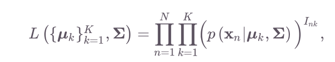
since

以来

Then, we plug in the Multivariate Normal PDF (dropping multiplicative constants) and take the log:

然后，我们插入多元正态PDF(删除乘法常数)并记录日志：

Finally, we have our data likelihood. Now we estimate the parameters by maximizing this expression.

最后，我们有数据可能性。 现在我们通过最大化该表达式来估计参数。

Let’s start with 𝚺. First, simplify the log-likelihood to make the gradient with respect to 𝚺 more apparent.

让我们从𝚺开始。 首先，简化对数似然以使相对于梯度Σ更加明显。

Then, we take the derivative. Note that this uses matrix derivatives (2) and (3) introduced in the “math note” here.

然后，我们取导数。 请注意，这使用此处 “数学笔记”中介绍的矩阵导数(2)和(3)。

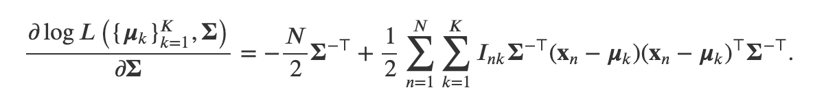
Then we set this gradient equal to 0 and solve for 𝚺.

然后我们将此梯度设置为0并求解𝚺。

where

哪里

Half way there! Now to estimate 𝝁_k (the kth class’s mean vector), let’s look at each class individually. Let C_k be the set of observations in class k. Looking only at terms involving 𝝁_k, we get

有一半！ 我们估计μ_K(第k个类的平均矢量)，单独让我们来看看每个类。 令C_k为类别k中的观测值集合。 只看涉及𝝁 _k的项，我们得到

Using equation (4) from the “math note” here, we get the gradient to be

使用此处 “数学笔记”中的方程式(4)，我们得到的梯度为

Finally, we set this gradient equal to 0 and find our estimate of the mean vector:

最后，我们将此梯度设置为0并找到我们对均值矢量的估计：

where the last term gives the sample mean of the x in class k.

最后一项给出类k中 x的样本均值。

3.2.2 Quadratic Discriminant Analysis (QDA)

3.2.2二次判别分析(QDA)

QDA looks very similar to LDA but assumes each class has its own covariance matrix. I.e.,

QDA看起来与LDA非常相似，但是假设每个类都有自己的协方差矩阵。 即

The log-likelihood is the same in LDA except we the 𝚺 with a 𝚺_k:

对数似然是LDA一样，除了我们用Σ_K的Σ：

Again, let’s look at the parameters for the kth class individually. The log-likelihood for class k is given by

再次，让我们分别查看第k个类的参数。 k类的对数似然由下式给出

We could take the gradient of this log-likelihood with respect to 𝝁_k and set it equal to 0 to solve for our estimate of 𝝁_k. However, we can also note that this estimate from the LDA approach will hold since this expression didn’t depend on the covariance term (which is the only thing we’ve changed). Therefore, we again get

我们可以利用这个数似然的梯度相对于μ_K和将其设置为0，以解决我们的估计 μ_K。 但是，我们也可以注意到，由于该表达式不取决于协方差项(这是我们唯一更改的项)，因此LDA方法的估计值将成立。 因此，我们再次得到

To estimate the 𝚺_k, we take the gradient of the log-likelihood for class k.

为了估计Σ_K，我们采取了数似然类k的梯度。

Then we set this equal to 0 to get our estimate:

然后，将其设置为等于0以获得估算值：

where

哪里

3.2.3 Naive Bayes

3.2.3朴素贝叶斯

Naive Bayes assumes the random variables within x are independent conditional on the class of the observation. That is, if x is D-dimensional,

朴素贝叶斯(Naive Bayes)假设x内的随机变量是独立于观察类别的条件。 也就是说，如果x是D维的，

This makes calculating p(x|y = k) very easy — to estimate the parameters of p(x[j]|y), we can ignore all variables in x other than the jth.

这使得计算p( x | y = k)非常容易-估计p( x [j] | y)的参数，我们可以忽略x中除第j个变量之外的所有变量。

As an example, suppose x is two-dimensional and we use the following model, where for simplicity σ is known.

例如，假设x是二维的，我们使用以下模型，其中为简单起见，σ是已知的。

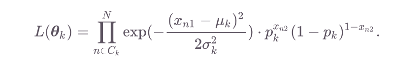
As before, we estimate the parameters in each class by looking only at the terms in that class. Let θ_k = (μ_k, σ_k, p_k) contain the relevant parameters for class k. The likelihood for class k is given by the following,

和以前一样，我们仅通过查看该类中的术语来估计每个类中的参数。 让θ_K =(μ_k，σ_k，P_K)包含类k的相关参数。 k类的可能性由下式给出：

where the two are equal due to the assumed independence between the entries in x. Subbing in the Normal and Bernoulli densities for x_n1 and x_n2, respectively, we get

由于x中条目之间的假定独立性，因此两者相等。 分别减去x_n1和x_n2的法线和伯努利密度，我们得到

Then we can take the log likelihood as follows

然后我们可以将对数似然性如下

Finally we’re ready to find our estimates. Taking the derivative with respect to p_k, we’re left with

最后，我们准备找到我们的估计。 取关于p_k的导数，我们剩下

which will give us the sensible result that

这将给我们明智的结果

Notice this is just the average of the x_2’s. The same process will give us the typical results for μ_k and σ_k.

请注意，这只是x_2的平均值。 相同的过程将为我们提供μ_k和σ_k的典型结果。

4.进行分类 (4. Making Classifications)

Regardless of our modeling choices for p(x|y = k), classifying new observations is easy. Consider a test observation x_0. For k = 1, 2, …, K, we use Bayes’ rule to calculate

无论我们为p( x | y = k)选择哪种建模方法，对新观测值进行分类都是很容易的。 考虑一个测试观察值x _0 。 对于k = 1，2，…，K ，我们使用贝叶斯法则来计算

where 𝑝̂ gives the estimated density of x_0 conditional on y_0. We then predict y_0 = k for whichever value k maximizes the above expression.

𝑝̂给出了以y_0为条件的x _0的估计密度。 然后我们预测y_0 = k ，无论哪个值k使上述表达式最大化。

结论 (Conclusion)

Generative models like LDA, QDA, and Naive Bayes are among the most common methods for classifications. However, the (albeit arduous) details of their fitting process are often swept under the rug. The aim of this article is to make those details clear.

LDA，QDA和朴素贝叶斯等生成模型是最常见的分类方法之一。 但是，其安装过程的细节(尽管很艰苦)经常被人扫了一下。 本文的目的是使这些细节清楚。

While the low-level details of estimating parameters for a generative model can be quite complex, the high-level intuition is quite straightforward. Let’s recap this intuition in a few simple steps.

虽然生成模型的参数估计的底层细节可能非常复杂，但高层直觉却非常简单。 让我们用几个简单的步骤来回顾一下这种直觉。

1. Estimate the prior probability that an observation is from any given class k. In math, estimate p(y = k) for each value of k.

   估计观察来自任何给定类别k的先验概率。 在数学中， 为k的每个值估计p(y = k) 。

2. Estimate the density of the predictors conditional on the observation’s class. I.e., estimate p(x|y = k) for each value of k.

   估计对观测的类条件的预测的密度。 即， 为k的每个值估计p( x | y = k) 。

3. Use Bayes’ Rule to obtain the probability that an observation is from any class given its predictors (up to a constant of proportionality): p(y = k|x).

   使用贝叶斯法则来获得观察值来自给定预测变量的任何类别的概率(最大比例常数)： p(y = k | x )。

4. Choose which value k maximizes the probability in step 3 (call it k*) and estimate that y = k*.

   在步骤3中选择哪个值k最大化概率(称为k *)，并估计y = k *。

And that’s it! To see more derivations from scratch like this one, please check out my free online book! I promise that most of them have less math.

就是这样！ 要查看从头开始的更多衍生内容，请查看我的免费在线书 ！ 我保证他们大多数人数学将减少。

翻译自: https://towardsdatascience.com/generative-classification-algorithms-from-scratch-d6bf0a81dcf7

fcn从头开始