


智能合约在衍生品上的应用
There is an overall skepticism in the job market with regard to machine learning engineers and their deep understanding of mathematics. The fact is, all machine learning algorithms are essentially mathematical frameworks — support-vector machines formulated as a dual optimization problem, principal component analysis as spectral decomposition filtering, or neural networks as a composition of successive non-linear functions — and only a thorough mathematical understanding will allow you to truly grasp them.
对于机器学习工程师及其对数学的深刻理解,就业市场总体上持怀疑态度。 事实是,所有机器学习算法本质上都是数学框架-支持向量机被表述为双重优化问题,主成分分析被表述为频谱分解滤波,或者神经网络被表述为连续的非线性函数的组成部分-仅是彻底的数学计算理解将使您真正地掌握它们。
Various Python libraries facilitate the usage of advanced algorithms to simple steps, e.g. Scikit-learn library with KNN, K-means, decision trees, etc., or Keras, that lets you build neural network architectures without necessarily understanding the details behind CNNs or RNNs. However, becoming a good machine learning engineer requires much more than that, and interviews for such positions often include questions on, for example, the implementation of KNN or decision trees from scratch or deriving the matrix closed-form solution of linear regression or softmax back-propagation equations.
各种Python库都有助于将高级算法用于简单的步骤, 例如带有KNN,K-means,决策树等的Scikit-learn库或Keras,可让您构建神经网络架构而不必了解CNN或RNN背后的细节。 。 但是,要成为一名优秀的机器学习工程师,不仅要做更多的工作,而且对此类职位的面试通常还涉及一些问题,例如,从头开始实施KNN或决策树,或者推导线性回归或softmax返回的矩阵封闭式解决方案。传播方程。
In this article, we will review some fundamental concepts of calculus — such as derivatives for uni- and multi-dimensional functions, including gradient, Jacobian and Hessian — to get you started with your interview preparation and, simultaneously, help you build a good foundation to successfully dive deeper into the exploration of mathematics behind machine learning, especially for neural networks.
在本文中,我们将回顾一些微积分的基本概念,例如一维和多维函数的导数,包括渐变, Jacobian和Hessian ,以帮助您开始面试准备,同时帮助您建立良好的基础成功地深入研究机器学习背后的数学探索,尤其是对于神经网络。
These concepts will be demonstrated with 5 examples of derivatives that you should absolutely have in your pocket for interviews:
这些概念将通过5个衍生品示例进行演示,您绝对应该在访谈中使用这些衍生品:
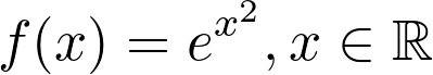
Derivative of a Composed Exponential Function — f(x)= eˣ ²
合成指数函数的导数— f(x)=eˣ²
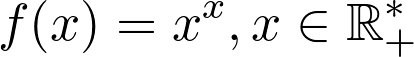
Derivative of a Variable Base and Variable Exponent Function — f(x)= xˣ
可变基数和可变指数函数的导数-f(x)=xˣ
Gradient of Multi-Dimensional Input Function — f(x,y,z) = 2ˣʸ+zcos(x)
多维输入函数的渐变— f(x,y,z)=2ˣʸ+ zcos(x)
Jacobian of a Multi-Dimensional Function — f(x,y) = [2x², x √y]
多维函数的雅可比行列式-f(x,y)= [2x²,x√y]
Hessian of a Multi-Dimensional Input Function — f(x,y) = x ²y³
多维输入函数的黑森州— f(x,y)= x²y³
导数1:合成指数函数 (Derivative 1: Composed Exponential Function)
The exponential function is a very foundational, common, and useful example. It is a strictly positive function, i.e. eˣ > 0 in ℝ, and an important property to remember is that e⁰ = 1. In addition, you should remember that the exponential is the inverse of the logarithmic function. It is also one of the easiest functions to derivate because its derivative is simply the exponential itself, i.e. (eˣ)’ = eˣ. The derivative becomes tricker when the exponential is combined with another function. In such cases, we use the chain rule formula, which states that the derivative of f(g(x)) is equal to f’(g(x))⋅g’(x), i.e.:
指数函数是一个非常基础,通用和有用的示例。 它是严格的正函数, 即ˣ中的eˣ> 0 ,并且要记住的一个重要属性是e⁰=1 。此外,您应记住,指数是对数函数的倒数。 它也是最容易推导的函数之一,因为它的导数就是指数本身, 即(eˣ)'=eˣ。 当指数与另一个函数结合时,导数会变得更加棘手。 在这种情况下,我们使用链式规则公式,该公式指出f(g(x))的导数等于f'(g(x))⋅g'(x) , 即 :

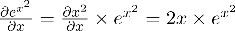
Applying chain rule, we can compute the derivative of f(x)= eˣ ². We first find the derivative of g(x)=x², i.e. g(x)’=2x. We also know that (eˣ)’=eˣ. Multiplying these two intermediate results, we obtain
应用链式规则,我们可以计算f(x)=eˣ²的导数。 我们首先找到g(x)=x²的导数,即g(x)'= 2x。 我们也知道( eˣ)'=eˣ。 这些相乘 我们得到两个中间结果
This is a very simple example that might seem trivial at first, but it is often asked by interviewers as a warmup question. If you haven’t seen derivatives for a while, make sure that you can promptly react to such simple problems, because while this won’t give you the job, failing on such a fundamental question could definitely cost you the job!
这是一个非常简单的示例,乍看之下似乎微不足道,但它经常被访调员问作为一个热身问题。 如果您已经有一段时间没有看到衍生产品了,请确保您可以对这些简单的问题Swift做出React,因为尽管这不能给您带来工作,但是在这样一个基本问题上的失败肯定会使您付出工作!
导数2.具有可变基数和可变指数的函数 (Derivative 2. Function with Variable Base and Variable Exponent)
This function is a classic in interviews, especially in the financial/quant industry, where math skills are tested in even greater depth than in tech companies for machine learning positions. It sometimes brings the interviewees out of their comfort zone, but really, the hardest part of this question is to be able to start correctly.
此功能是面试中的经典之作,尤其是在金融/定量行业中,在该行业中,对数学技能的测试甚至比在高科技公司中对机器学习职位的测试还要深入。 有时这会使受访者脱离他们的舒适范围,但实际上,这个问题最难的部分是能否正确开始。
The most important thing to realize when approaching a function in such exponential form is, first, the inverse relationship between exponential and logarithm, and, second, the fact, that every exponential function can be rewritten as a natural exponential function in the form of
当以这种指数形式接近函数时,要实现的最重要的事情是,首先,指数与对数之间成反比关系,其次,事实是,每个指数函数都可以重写为自然指数函数,形式为

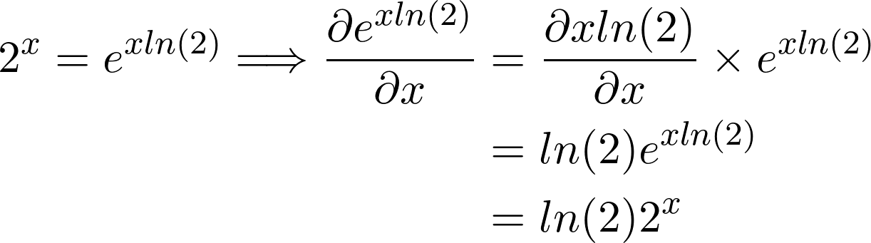
Before we get to our f(x) = xˣ example, let us demonstrate this property with a simpler function f(x) = 2ˣ. We first use the above equation to rewrite 2ˣ as exp(xln(2)) and subsequently apply chain rule to derivate the composition.
在进入f(x)=xˣ示例之前,让我们用一个更简单的函数f(x)=2ˣ演示此属性。 我们首先使用以上等式重写2ˣ为exp(XLN(2)),并且随后应用链式法则,推导所述组合物。
Going back to the original function f(x)=xˣ, once you rewrite the function as f(x)=exp(x ln x), the derivative becomes relatively straightforward to compute, with the only potentially difficult part being the chain rule step.
回到原始函数f(x)=xˣ ,一旦将函数重写为f(x)= exp(x ln x) ,则导数变得相对容易计算,唯一可能的困难部分是链规则步骤。
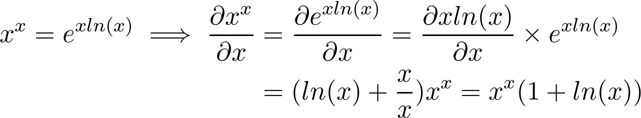
Note that here we used the product rule (uv)’=u’v+uv’ for the exponent xln(x).
请注意,这里我们对指数xln(x)使用乘积规则(uv)'= u'v + uv' 。
This function is generally asked without any information on the function’s domain. If your interviewer doesn’t specify the domain by default, he might be testing your mathematical acuity. Here is where the question gets deceiving. Without being specific about the domain, it seems that xˣ is defined for both positive and negative values. However, for negative x, e.g.(-0.9)^(-0.9), the result is a complex number, concretely -1.05–0.34i. A potential way out would be to define the domain of the function as ℤ⁻ ∪ ℝ⁺ \0 (see here for further discussion), but this would still not be differentiable for negative values. Therefore, in order to properly define the derivative of xˣ, we need to restrict the domain to only strictly positive values. We exclude 0 because for a derivative to be defined in 0, we need the limit derivative from the left (limit in 0 for negative values) to be equal to the limit derivative from the right (limit in 0 for positive values) — a condition that is broken in this case. Since the left limit
通常在没有该功能域的任何信息的情况下询问此功能。 如果您的面试官默认情况下未指定域,则他可能正在测试您的数学敏锐度。 这是骗人的地方。 无需具体说明域,似乎xˣ被定义为正值和负值。 但是,对于负x , 例如(-0.9)^(-0.9) ,结果是一个复数,具体是-1.05-0.34i 。 可能的解决方法是将函数的域定义为ℝ⁺\ 0(请参见此处进一步讨论),但这对于负值仍然不可区分。 因此,为了正确定义xˣ的导数,我们需要将域限制为严格的正值。 我们排除0是因为要在0中定义一个导数,我们需要从左边开始的极限导数(对于负值,极限为0)等于从右边开始的极限导数(对于正值,极限为0)—一个条件在这种情况下是坏的。 自左极限

is undefined, the function is not differentiable in 0, and thus the function’s domain is restricted to only positive values.
为undefined时,该函数不可微分为0,因此该函数的域仅限于正值。
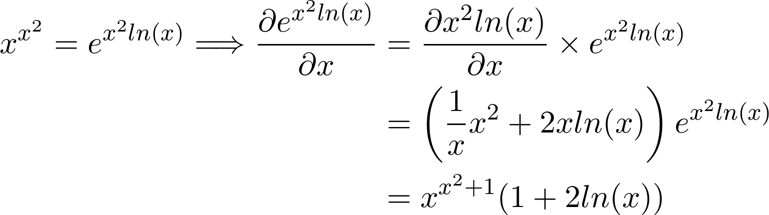
Before we move on to the next section, I leave you with a slightly more advanced version of this function to test your understanding: f(x) = xˣ². If you understood the logic and steps behind the first example, adding the extra exponent shouldn’t cause any difficulties and you should conclude the following result:
在继续进行下一部分之前,我为您提供此功能的稍高版本,以测试您的理解: f(x)= x = ²。 如果您了解第一个示例的逻辑和步骤,那么添加额外的指数应该不会造成任何困难,并且应该得出以下结果:
导数3:多维输入函数的梯度 (Derivative 3: Gradient of a Multi-Dimensional Input Function)

So far, the functions discussed in the first and second derivative sections are functions mapping from ℝ to ℝ, i.e. the domain as well as the range of the function are real numbers. But machine learning is essentially vectorial and the functions are multi-dimensional. A good example of such multidimensionality is a neural network layer of input size m and output size k, i.e. f(x) = g(Wᵀx + b), which is an element-wise composition of a linear mapping Wᵀx (with weight matrix W and input vector x) and a non-linear mapping g (activation function). In the general case, this can also be viewed as a mapping from ℝᵐ to ℝᵏ.
到目前为止,在第一和第二导数部分讨论的函数是从ℝ映射到ℝ的函数, 即函数的域和范围都是实数。 但是机器学习本质上是矢量的,其功能是多维的。 这种多维性的一个很好的例子是输入大小为m而输出大小为k的神经网络层,即f(x)= g(Wᵀx+ b),其中 是线性映射Wᵀx(具有权重矩阵W和输入向量x )和非线性映射g (激活函数)的逐元素组合。 在一般情况下,这也可以视为从ℝᵐ到ℝᵏ的映射。
In the specific case of k=1, the derivative is called gradient. Let us now compute the derivative of the following three-dimensional function mapping ℝ³ to ℝ:
在k = 1的特定情况下,导数称为梯度 。 现在让我们来计算下的三维功能映射ℝ³到的导数 ℝ:

You can think of f as a function mapping a vector of size 3 to a vector of size 1.
您可以将f视为将大小为3的向量映射为大小为1的向量的函数。
The derivative of a multi-dimensional input function is called a gradient and is denoted by the symbol nabla (inverted delta): ∇. A gradient of a function g that maps ℝⁿ to ℝ is a set of n partial derivatives of g where each partial derivative is a function of n variables. Thus, if g is a mapping from ℝⁿ to ℝ, its gradient ∇g is a mapping from ℝⁿ to ℝⁿ.
多维输入函数的导数称为梯度 ,并用符号nabla (反向delta )表示。 函数g的梯度 映射ℝⁿ到ℝ是g的n个偏导数的集合,其中每个偏导数都是n个变量的函数。 因此,如果g是从ℝⁿ到ℝ的映射,则其梯度∇g是从ℝⁿ到ℝⁿ的映射。
To find the gradient of our function f(x,y,z) = 2ˣʸ + zcos(x), we construct a vector of partial derivatives ∂f/∂x, ∂f/∂y and ∂f/∂z, and obtain the following result:
为了找到函数f(x,y,z)=2ˣʸ+ zcos(x)的梯度,我们构造了偏导数∂f/∂x,∂f/∂y和∂f/ ∂z的向量,并获得结果如下:
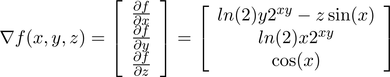
Note that this is an example similar to the previous section and we use the equivalence 2ˣʸ=exp(xy ln(2)).
请注意,这是一个与上一节相似的示例,我们使用等价2ˣʸ= exp(xy ln(2))。
In conclusion, for a multi-dimensional function that maps ℝ³ to ℝ, the derivative is a gradient ∇ f, which maps ℝ³ to ℝ³.
总之,对于映射ℝ³到多维函数 ℝ,该衍生物是梯度∇F,其映射到ℝ³ℝ³。
In a general form of mappings ℝᵐ to ℝᵏ where k > 1, the derivative of a multi-dimensional function that maps ℝᵐ to ℝᵏ is a Jacobian matrix (instead of a gradient vector). Let us investigate this in the next section.
在将k映射为>的 a的通用形式中,将ℝᵐ映射到multi的多维函数的导数是雅可比矩阵(而不是梯度矢量)。 让我们在下一部分中对此进行调查。
导数4.多维输入和输出函数的雅可比行列式 (Derivative 4. Jacobian of a Multi-Dimensional Input and Output Function)
We know from the previous section that the derivative of a function mapping ℝᵐ to ℝ is a gradient mapping ℝᵐ to ℝᵐ. But what about the case where also the output domain is multi-dimensional, i.e. a mapping from ℝᵐ to ℝᵏ for k>1?
从上一节我们知道,函数映射到的导数是梯度映射到。 但是,如果输出域也是多维的, 即 k> 1时从ℝᵐ到mapping的映射,该怎么办?
In such case, the derivative is called Jacobian matrix. We can view gradient simply as a special case of Jacobian with dimension m x 1 with m equal to the number of variables. The Jacobian J(g) of a function g mapping ℝᵐ to ℝᵏ is a mapping of ℝᵐ to ℝᵏ*ᵐ. This means that the output domain has a dimension of k x m, i.e. is a matrix of shape k x m. In other words, each row i of J(g) represents the gradient ∇ gᵢ of each sub-function gᵢ of g.
在这种情况下,导数称为Jacobian矩阵 。 我们可以简单地将梯度看作是Jacobian的特例,其维度为m x 1 , m等于变量数。 函数g映射ℝᵐ到ℝᵏ的Jacobian J(g)是ℝᵐ到ℝᵏ*ᵐ的映射。 这意味着输出域的尺寸为k x m , 即形状为k x m的矩阵。 换句话说,J(G)的每一行i表示梯度∇ 克的每个子功能gᵢ的gᵢ。
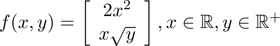
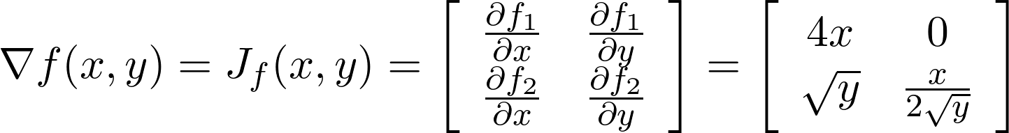
Let us derive the above defined function f(x, y) = [2x², x √y] mapping ℝ² to ℝ², thus both input and output domains are multidimensional. In this particular case, since the square root function is not defined for negative values, we need to restrict the domain of y to ℝ⁺. The first row of our output Jacobian will be the derivative of function 1, i.e.∇ 2x², and the second row the derivative of function 2, i.e. ∇ x √y.
让我们导出上面定义的函数f(x,y)= [2x²,x√y]映射 ℝ²到ℝ²,因此输入和输出域都是多维的。 在这种特殊情况下,由于未为负值定义平方根函数,因此我们需要将y的域限制为ℝ⁺。 输出雅可比行列的第一行将是函数1的导数, 即∇2x²,第二行是函数2的导数, 即 ∇x√y。
In deep learning, an example where the Jacobian is of special interest is in the explainability field (see, for example, Sensitivity based Neural Networks Explanations) that aims to understand the behavior of neural networks and analyses sensitivity of the output layer of neural networks with regard to the inputs. The Jacobian helps to investigate the impact of variation in the input space on the output. This can analogously be applied to understand the concepts of intermediate layers in neural networks.
在深度学习中,Jacobian特别令人关注的一个示例是在可解释性领域(例如,参见基于灵敏度的神经网络解释 ),该示例旨在了解神经网络的行为并分析神经网络输出层的灵敏度。关于输入。 雅可比矩阵有助于研究输入空间中的变化对输出的影响。 可以类似地将其应用于理解神经网络中的中间层的概念。
In summary, remember that while gradient is a derivative of a scalar with regard to a vector, Jacobian is a derivative of a vector with regard to another vector.
总之,请记住,虽然梯度是向量的标量的导数,但雅可比矩阵是向量相对于另一个向量的导数。
导数5。多维输入函数的粗麻布 (Derivative 5. Hessian of a Multi-Dimensional Input Function)

So far, our discussion has only been focused on first-order derivatives, but in neural networks we often talk about higher-order derivatives of multi-dimensional functions. A specific case is the second derivative, also called the Hessian matrix, and denoted H(f) or ∇ ² (nabla squared) .The Hessian of a function g mapping ℝⁿ to ℝ is a mapping H(g) from ℝⁿ to ℝⁿ*ⁿ.
到目前为止,我们的讨论仅集中于一阶导数,但是在神经网络中,我们经常谈论多维函数的高阶导数。 一种特殊情况是二阶导数,也称为Hessian矩阵 ,表示为H(f)或∇²(nabla平方)。 函数g映射ℝⁿ到ℝ的Hessian是从ℝⁿ到ℝⁿ*ⁿ的映射H(g) 。
Let us analyze how we went from ℝ to ℝⁿ*ⁿ on the output domain. The first derivative, i.e. gradient ∇g, is a mapping from ℝⁿ to ℝⁿ and its derivative is a Jacobian. Thus, the derivation of each sub-function ∇gᵢ results in a mapping of ℝⁿ to ℝⁿ, with n such functions. You can think of this as if deriving each element of the gradient vector expanded into a vector, becoming thus a vector of vectors, i.e. a matrix.
让我们分析一下在输出域上从ℝ到ℝⁿ*ⁿ的过程。 一阶导数, 即梯度,是从到的映射,其导数是雅可比行列式。 因此,每个子函数∇g的推导导致ℝⁿ到ℝⁿ的映射,其中n个这样的函数。 您可以认为这就像将梯度向量的每个元素都扩展为向量一样,从而成为向量的向量, 即矩阵。
To compute the Hessian, we need to calculate so-called cross-derivatives, that is, derivate first with respect to x and then with respect to y, or vice-versa. One might ask if the order in which we take the cross derivatives matters; in other words, if the Hessian matrix is symmetric or not. In cases where the function f is 𝒞², i.e. twice continuously differentiable, Schwarz theorem states that the cross derivatives are equal and thus the Hessian matrix is symmetric. Some discontinuous, yet differentiable functions, do not satisfy the equality of cross-derivatives.
为了计算Hessian,我们需要计算所谓的交叉导数,即,首先是相对于x然后是相对于y的导数 ,反之亦然。 有人可能会问我们采用交叉导数的顺序是否重要? 换句话说,Hessian矩阵是否对称。 在函数f为𝒞²的情况下, 即两次连续可微化, Schwarz定理指出交叉导数相等,因此Hessian矩阵是对称的。 一些不连续但可微的函数不能满足交叉导数的相等性。
Constructing the Hessian of a function is equal to finding second-order partial derivatives of a scalar-valued function. For the specific example f(x,y) = x²y³, the computation yields the following result:
构造函数的Hessian等于找到标量值函数的二阶偏导数。 对于特定示例f(x,y)=x²y³ ,计算得出以下结果:
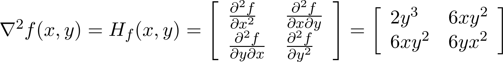
You can see that the cross-derivatives 6xy² are in fact equal. We first derived with regard to x and obtained 2xy³, then again with regard to y, obtaining 6xy². The diagonal elements are simply fᵢ” for each mono-dimensional sub-function of either x or y.
您会看到交叉导数6xy²实际上是相等的。 我们首先关于x推导得出2xy³,然后关于y 得出6xy²。 对角元素是简单地fᵢ”为x或y中的每个单维子功能。
An extension would be to discuss the case of a second order derivatives for multi-dimensional functions mapping ℝᵐ to ℝᵏ, which can intuitively be seen as a second-order Jacobian. This is a mapping from ℝᵐ to ℝᵏ*ᵐ*ᵐ, i.e. a 3D tensor. Similarly to the Hessian, in order to find the gradient of the Jacobian (differentiate a second time), we differentiate each element of the k x m matrix and obtain a matrix of vectors, i.e. a tensor. While it is rather unlikely that you would be asked to do such computation manually, it is important to be aware of higher-order derivatives for multidimensional functions.
扩展将是讨论用于将functions映射到ℝᵏ的多维函数的二阶导数的情况,直觉上可以将其视为二阶雅可比矩阵。 这是从ℝᵐ到ℝᵏ*ᵐ*ᵐ( 即 3D张量)的映射。 与Hessian相似,为了找到Jacobian梯度(第二次求差),我们对k x m矩阵的每个元素求微分,并获得矢量矩阵, 即张量。 尽管不太可能会要求您手动进行此类计算,但重要的是要了解多维函数的高阶导数。
结论 (Conclusion)
In this article, we reviewed important calculus fundamentals behind machine learning. We demonstrated them with examples of uni- and multidimensional functions, discussing gradient, Jacobian, and Hessian. This review is a thorough walk-through of possible interview concepts and an overview of calculus-related knowledge behind machine learning.
在本文中,我们回顾了机器学习背后的重要演算基础。 我们用一维和多维函数的示例对其进行了演示,讨论了梯度,雅可比和黑森州。 这篇评论是对可能的面试概念的彻底演练,并概述了机器学习背后与微积分相关的知识。
智能合约在衍生品上的应用


 1万+
1万+

 被折叠的 条评论
为什么被折叠?
被折叠的 条评论
为什么被折叠?
 到【灌水乐园】发言


