


 本文探讨了在资源受限的空间环境中部署深度学习模型时面临的挑战,并介绍了几种有效的模型压缩技术,包括修剪、量化、低秩近似、知识蒸馏及神经架构搜索。
太空夜景
By Hannah Peterson and George Williams (gwilliams@gsitechnology.com)
汉娜·彼得森 ( Hannah Peterson)和 乔治·威廉姆斯 ( George Williams) (gwilliams@gsitechnology.com)
空间计算 (Computing in space)
Every day we depend on extraterrestrial devices to send us information about the state of the Earth and surrounding space—currently, there are about 3,000 satellites orbiting the Earth and this number is growing rapidly. Processing and transmitting the wealth of data these devices produce is not a trivial task, given that resources in space such as on-board memory and downlink bandwidth face tight constraints. In the case of satellite images, the data at hand can be extremely large, sometimes as large as 8,000×8,000 pixels. For most practical applications, only part of the great amount of detail encoded in these images is of interest—such as the footprints of buildings, for example—but the current standard approach is to transmit the entire images back to Earth for processing. It seems a more efficient solution would be to process the data on board the spacecraft, arriving at a compressed representation that occupies fewer resources—something that could be achieved using a machine learning model.
每天,我们都依靠外星设备向我们发送有关地球状态和周围空间状态的信息-当前,大约有3,000颗卫星绕地球旋转,并且这一数字正在Swift增长。 考虑到空间资源(如板载内存和下行链路带宽)面临严格的约束,处理和传输这些设备产生的大量数据并非易事。 在卫星图像的情况下,手头的数据可能非常大,有时甚至高达8,000×8,000像素。 对于大多数实际应用而言,这些图像中编码的大量细节中只有一部分是令人感兴趣的,例如建筑物的足迹,但是当前的标准方法是将整个图像传输回地球进行处理。 似乎更有效的解决方案是在航天器上处理数据,从而获得占用更少资源的压缩表示形式,这可以使用机器学习模型来实现。
Unfortunately, running machine learning models tends to be a resource-intensive process even here on Earth. State-of-the-art networks typically consist of many millions of parameters and limited uplink bandwidth makes uploading such large networks to satellites impractical/infeasible. And even if they were pre-loaded prior to launch, they require significant memory bandwidth to fetch weights and compute dot products at runtime. Energy consumption of these networks is dominated by memory accesses, and they typically rely on hardware accelerators for timely inference. Spacecraft, however, face very strict weight and power requirements, which means that a satellite can’t be loaded with an unlimited number of GPUs for the purpose of running a model.
不幸的是,即使在地球上,运行机器学习模型也往往是资源密集型过程。 最先进的网络通常包含数百万个参数,而有限的上行链路带宽使得将如此大型的网络上传到卫星是不切实际/不可行的。 即使它们在启动前已预先加载,它们也需要大量内存带宽才能在运行时获取权重并计算点积。 这些网络的能耗主要由内存访问决定,它们通常依赖硬件加速器进行及时推断。 但是,航天器面临非常严格的重量和功率要求,这意味着,为了运行模型,不能为卫星装载无限数量的GPU。
In this way, the topic of model compression is particularly relevant to space-based applications, as there is an evident need to reduce the size and complexity of neural networks for deployment in highly constrained extraterrestrial environments. Luckily, many effective techniques for model compression exist thanks to a rapidly growing body of research on the topic. In this blog, I’ll be going over a few common approaches.
以此方式, 模型压缩的主题与基于空间的应用特别相关,因为显然需要减小神经网络的大小和复杂性,以便在高度受限的外星环境中进行部署。 幸运的是,由于有关该主题的研究Swift增长,因此存在许多有效的模型压缩技术。 在此博客中,我将介绍一些常用方法。
什么是模型压缩? (What is model compression?)
The goal of model compression is to achieve a model that is simplified from the original without significantly diminished accuracy. A simplified model is one that is reduced in size and/or latency from the original. Specifically, a size reduction means that the compressed model has fewer and/or smaller parameters and, thus, uses less RAM when run, which is desirable because it frees up memory for other parts of the application to use. A latency reduction is a decrease in the time it takes for the model to make a prediction, or inference, based on an input to the trained model, typically translating to lower energy consumption at runtime. Model size and latency often go hand-in-hand because larger models require more memory accesses to be run. As we can see, both types of reduction are desirable for deploying models in space, where computing resources face both strict size and power constraints.
模型压缩的目的是要实现一种从原始模型简化而又没有明显降低精度的模型。 简化模型是一种在尺寸和/或等待时间方面都比原始模型减少的模型。 具体而言, 减小大小意味着压缩的模型具有越来越少的参数,因此在运行时使用更少的RAM,这是理想的,因为它释放了内存供应用程序的其他部分使用。 延迟减少是指模型根据训练后的模型的输入来进行预测或推理所需的时间减少,通常可以在运行时降低能耗。 模型大小和延迟通常是并行的,因为较大的模型需要运行更多的内存访问权限。 正如我们所看到的,两种减少类型都适合在空间中部署模型,因为在这些空间中计算资源面临严格的大小和功耗约束。
The following are some popular, heavily researched methods for achieving compressed models:
以下是一些流行的,经过深入研究的用于实现压缩模型的方法:
- Pruning 修剪
- Quantization 量化
- Low-rank approximation and sparsity 低秩近似和稀疏
- Knowledge distillation 知识升华
- Neural Architecture Search (NAS) 神经架构搜索(NAS)
Let’s take a look at each technique individually. In practice, a complete model compression pipeline might integrate several of these approaches, as each comes with its own benefits and drawbacks.
让我们分别看一下每种技术。 实际上,一个完整的模型压缩管道可能会集成其中的几种方法,因为每种方法都有其自身的优缺点。
修剪 (Pruning)
Pruning involves removing connections between neurons or entire neurons, channels, or filters from a trained network, which is done by zeroing out values in its weights matrix or removing groups of weights entirely; for example, to prune a single connection from a network, one weight is set to zero in a weights matrix, and to prune a neuron, all values of a column in a matrix are set to zero. The motivation behind pruning is that networks tend to be over-parametrized, with multiple features encoding nearly the same information. Pruning can be divided into two types based on the type of network component being removed: unstructured pruning involves removing individual weights or neurons, while structured pruning involves removing entire channels or filters. We’ll look at these two types individually, as they differ in their implementations and outcomes.
修剪涉及从受过训练的网络中删除神经元或整个神经元,通道或过滤器之间的连接,这是通过将其权重矩阵中的值清零或完全删除权重组来完成的; 例如,为了修剪来自网络的单个连接,在权重矩阵中将一个权重设置为零,并且为了修剪神经元,将矩阵中一列的所有值都设置为零。 修剪背后的动机是网络往往被过度参数化,多个功能对几乎相同的信息进行编码。 根据要删除的网络组件的类型,修剪可以分为两种类型: 非结构化修剪涉及删除单个权重或神经元,而结构化修剪涉及删除整个通道或过滤器。 我们将分别研究这两种类型,因为它们的实现和结果不同。
非结构化修剪 (Unstructured Pruning)

By replacing connections or neurons with zeros in a weights matrix, unstructured pruning increases the sparsity of the network, i.e. its proportion of zero to non-zero weights. There exist various hardware and software, such as TensorFlow Lite and Caffe, that are specialized to efficiently load and perform operations on sparse matrices and, thus, that can facilitate significant latency reductions in pruned models as compared to their original dense representations. For example, Caffe can be used to apply a mask to pruned parameters that causes them to be skipped over during network operation, reducing the amount of FLOPs and, thus, the power and time, required to make an inference. Depending on the degree of sparsity and the method of storage used, pruned networks can also take up much less memory than their dense counterparts.
通过在权重矩阵中将连接或神经元替换为零,非结构化修剪会增加网络的稀疏度,即其权重在零与非零之间的比例。 存在各种硬件和软件,例如TensorFlow Lite和Caffe ,这些硬件和软件专用于在稀疏矩阵上有效地加载和执行操作,因此与原始的密集表示相比,可以大大减少修剪后的模型中的延迟。 例如,Caffe可以用于对修剪的参数应用掩码,从而使它们在网络运行期间被跳过,从而减少了FLOP的数量,从而减少了进行推理所需的功能和时间。 根据稀疏程度和使用的存储方法,修剪后的网络所占用的内存也要比密集的网络少得多。
But what is the criteria for deciding which weights should be removed? One common method known as magnitude-based pruning compares the weights’ magnitudes to a threshold value. A highly cited 2015 paper by Han et al. prompted widespread adoption of this approach. In their implementation, pruning is applied layer-by-layer. First, a predetermined “quality parameter” is multiplied by the standard deviation of a layer’s weights to calculate the threshold value and weights with magnitudes below the threshold are zeroed. After all layers are pruned, the model is retrained so that the remaining weights can adjust to compensate for those that were removed, and the process is repeated for several iterations. The researchers used this method to prune four different model architectures, two pre-trained on the MNIST dataset and two on the ImageNet dataset. We can see the effects of their unstructured pruning approach visualized in the following image, which shows the sparsity pattern of the first fully-connected layer for one of the MNIST networks, where the blue dots represent non-zero parameters:
但是,决定删除哪些权重的标准是什么? 一种称为基于幅度的修剪的常见方法将权重的幅度与阈值进行比较。 Han等人在2015年发表的论文被高度引用。 促使该方法被广泛采用。 在其实现中,修剪是逐层应用的。 首先,将预定的“质量参数”乘以层权重的标准偏差以计算阈值,并将幅度低于阈值的权重置零。 修剪完所有图层后,对模型进行重新训练,以便可以调整其余权重以补偿已删除的权重,并且重复此过程几次迭代。 研究人员使用这种方法修剪了四种不同的模型架构,其中两种在MNIST数据集上进行了预训练,另外两种在ImageNet数据集上进行了训练。 我们可以在下图中直观地看到其非结构化修剪方法的效果,该图显示了一个MNIST网络的第一个完全连接层的稀疏模式,其中蓝色点表示非零参数:

The MNIST dataset consists of 28×28 pixel images of handwritten digits from 0–9 like the one above and models are trained to classify these digits. To be inputted into a neural network, the image is flattened by concatenating the rows of pixels end-to-end from top to bottom, resulting in a vector of 784 values. The first layer of the network is fully-connected with 300 neurons. As we can see, the digits tend to be oriented in the center of the image, thus pixels around the edges are less consequential to the classification task and connections to them get pruned more heavily. For the entire network, pruning caused both the number of non-zero weights and FLOPs required to decrease by a factor of 12 with no drop in predictive performance. Similarly, for the AlexNet and VGG-16 models trained on ImageNet, the numbers of parameters were reduced from 61 million to 6.7 million and from 138 million to 10.3 million, respectively, with no decrease in classification accuracy.
MNIST数据集由28至28像素的手写数字组成,从0到9,与上述数字相同,并且训练了模型来对这些数字进行分类。 要输入到神经网络中,可以通过从上到下端对端连接像素行来使图像变平,从而得到784个值的向量。 网络的第一层与300个神经元完全连接。 正如我们所看到的,数字倾向于定位在图像的中心,因此边缘周围的像素对分类任务的影响较小,并且与它们的连接被更大量地修剪。 对于整个网络,修剪会导致非零权重数和所需的FLOP减少12倍,而预测性能不会下降。 同样,对于在ImageNet上训练的AlexNet和VGG-16模型,参数的数量分别从6100万减少到670万,从1.38亿减少到1030万,而分类精度没有降低。
Han et. al showed that when implemented correctly, unstructured pruning can yield some truly impressive degrees of compression, as they note “the storage requirements of AlexNet and VGGNet are are small enough that all weights can be stored on chip, instead of off-chip DRAM which takes orders of magnitude more energy to access.” However, they also acknowledge the “limitation of general purpose hardware on sparse computation” and, thus, use specialized software to work around this problem. Indeed, unstructured pruning’s reliance on specially designed software or hardware to handle network sparsity to speed up computations is a significant limitation, one that is not faced by taking a structured approach.
韩等 al等人指出,正确实施后,非结构化修剪会产生一定程度的压缩效果,因为他们指出“ AlexNet和VGGNet的存储要求非常小,可以将所有权重存储在芯片上,而无需使用片外DRAM。数量级以上的能源可供使用。” 但是,他们也承认“通用硬件在稀疏计算上的局限性”,因此使用专用软件来解决此问题。 的确,非结构化修剪依赖于专门设计的软件或硬件来处理网络稀疏性以加快计算速度是一个重大限制,而采用结构化方法并不会遇到这种限制。
结构化修剪 (Structured Pruning)

Unlike unstructured pruning, structured pruning does not result in weight matrices with problematic sparse connectivity patterns because it involves removing entire blocks of weights within given weight matrices. This means the pruned model can be run using the same hardware and software as the original. While we are now looking at groups of weights to remove at the channel or filter level, magnitude-based pruning can still be applied by ranking them according to their L1 norms, for example. But there are also more intelligent, “data-driven” approaches that have been proposed which can achieve better results.
与非结构化修剪不同,结构化修剪不会导致权重矩阵具有问题的稀疏连接模式,因为它涉及在给定权重矩阵内删除整个权重块。 这意味着可以使用与原始模型相同的硬件和软件来运行修剪的模型。 现在,我们正在研究要在通道或滤波器级别上删除的权重组,例如,仍然可以通过根据它们的L1规范对它们进行排序来应用基于幅度的修剪。 但是,还提出了更智能的“数据驱动”方法,可以实现更好的结果。
Huang et al., for example, were the first to integrate into the pruning process a means of controlling the tradeoff between network performance and size in their 2018 paper. Their algorithm outputs a set of filter “pruning agents”—each a neural network corresponding to a convolutional layer of the network—and an alternative, pruned version of the original model, which is initialized to be the same as the original. The pruning agents work to maximize an objective that is parametrized by a “drop bound” value, which is defined as the maximum allowed drop in performance between the original and the pruned model, forcing the agents to keep performance above a specified level. For each convolutional layer, a pruning agent is trained by evaluating the effects of pruning combinations of different filters within that layer. To do so, it removes certain filters from the alternative model and compares this model’s performance on an evaluation set to that of the original, learning which modifications will increase the network’s efficiency while still adhering to accuracy constraints. Once the agent for one layer is trained and filters for that layer have been optimally removed, the entire pruned model is retrained to adjust for the changes and the process repeats for the next convolutional layer.
例如,Huang等人在其2018年的论文中率先将修剪网络中的一种控制网络性能和规模之间权衡的方法集成到了修剪过程中。 他们的算法输出一组过滤器“修剪代理”(每个神经网络对应于该网络的卷积层),以及原始模型的另一种修剪版本,该版本被初始化为与原始模型相同。 修剪代理的工作是使由“下降界限”值参数化的目标最大化,该值定义为原始模型和修剪模型之间的最大允许性能下降,从而迫使代理将性能保持在指定水平以上。 对于每个卷积层,通过评估该层中不同过滤器的修剪组合的效果来训练修剪剂。 为此,它从替代模型中删除了某些过滤器,并将该模型在评估集上的性能与原始模型的性能进行了比较,从而了解了哪些修改将提高网络的效率,同时仍然遵守准确性约束。 一旦对一层的代理进行了训练,并已最佳地除去了该层的过滤器,就可以对整个修剪的模型进行再训练以针对更改进行调整,并且对下一个卷积层重复此过程。
The following plot shows the degree of pruning achieved with this approach with drop bound b = 2 on the layers of a VGG-16 model trained on the CIFAR 10 dataset. The greater degree of pruning of higher layers indicates they tend to contain more unnecessary filters than initial ones.
下图显示了这种方法在下降限制b = 2时达到的修剪程度 在CIFAR 10数据集上训练的VGG-16模型的层上。 较高层的修剪程度越高,表明它们倾向于包含比初始过滤器更多的不必要过滤器。

We can also see the quantitative compression results of pruning this model using different drop bound values. The accuracy values in parentheses correspond to models pruned to the same ratio but with a magnitude-based approach instead, and we see that the “data-driven” implementation has superior performance.
我们还可以看到使用不同的下降绑定值修剪此模型的定量压缩结果。 括号中的精度值对应于修剪成相同比率但使用基于幅度的方法的模型,并且我们看到“数据驱动”实现具有优越的性能。

Similarly impressive results have been achieved through a variety of structured pruning methods, establishing it as a popular model compression technique. But pruning in general still has a few potential drawbacks. For example, it’s generally unclear how well given methods generalize across different architectures, and the pruning process tends to involve a lot of fine-tuning that can act as a barrier both to implementation and generalization. Further, in many cases it may be more effective to simply use a more efficient architecture than to prune a suboptimal one. If you’re interested in taking a closer look at the diverse range of approaches currently being taken to prune models, I suggest checking out this blog or the paper “What is the State of Neural Network Pruning?”, both written in 2019.
同样,通过多种结构化修剪方法也获得了令人印象深刻的结果,并将其确立为流行的模型压缩技术。 但是修剪通常仍具有一些潜在的缺点。 例如,通常不清楚给定方法在不同体系结构上的推广程度如何,并且修剪过程往往涉及许多微调,这可能会阻碍实现和推广。 此外,在许多情况下,简单地使用更有效的体系结构可能比修剪次优的体系结构更为有效。 如果您有兴趣仔细研究当前用于修剪模型的各种方法,建议您查看此博客或论文“神经网络修剪的状态是什么?”。 ,均写于2019年。
量化 (Quantization)

While pruning compresses models by reducing the number of weights, quantization consists of decreasing the size of the weights that are there. Quantization in general is the process of mapping values from a large set to values in a smaller set, meaning that the output consists of a smaller range of possible values than the input, ideally without losing too much information in the process. We can think about this in the context of image compression, as with the images of Einstein above. In the leftmost representation, each pixel value is represented by 8 bits and thus can take on 256 varying shades of gray. The number of possible shades is halved in each successive image. Notice, however, that we really aren’t able to detect much difference between the first four images or so, and this represents the goal of model quantization: to reduce the precision of network components to the extent that it is more lightweight but without a “noticeable” difference in efficacy. Intuitively, it makes sense that neural networks should be able to deal with some information loss, as they are trained to cope well with high levels of noise in their inputs, and lower precision calculations can essentially be seen as another source of noise.
修剪通过减少权数来压缩模型时,量化包括减小权重的大小。 通常,量化是将值从较大的集合映射到较小的集合中的值的过程,这意味着输出包含比输入更小的范围的可能值,理想情况下不会丢失太多信息。 我们可以在图像压缩的情况下考虑这一点,就像上面的爱因斯坦的图像一样。 在最左边的表示中,每个像素值由8位表示,因此可以采用256种不同的灰色阴影。 在每个连续的图像中,可能的阴影数量减半。 但是请注意,我们实际上无法检测出大约前四个图像之间的差异,这代表了模型量化的目标:将网络组件的精度降低到更轻量但没有功效“明显”差异。 从直觉上讲,神经网络应该能够处理一些信息丢失,因为它们经过训练可以很好地应对输入中的高水平噪声,而精度较低的计算本质上可以看作是另一种噪声源。
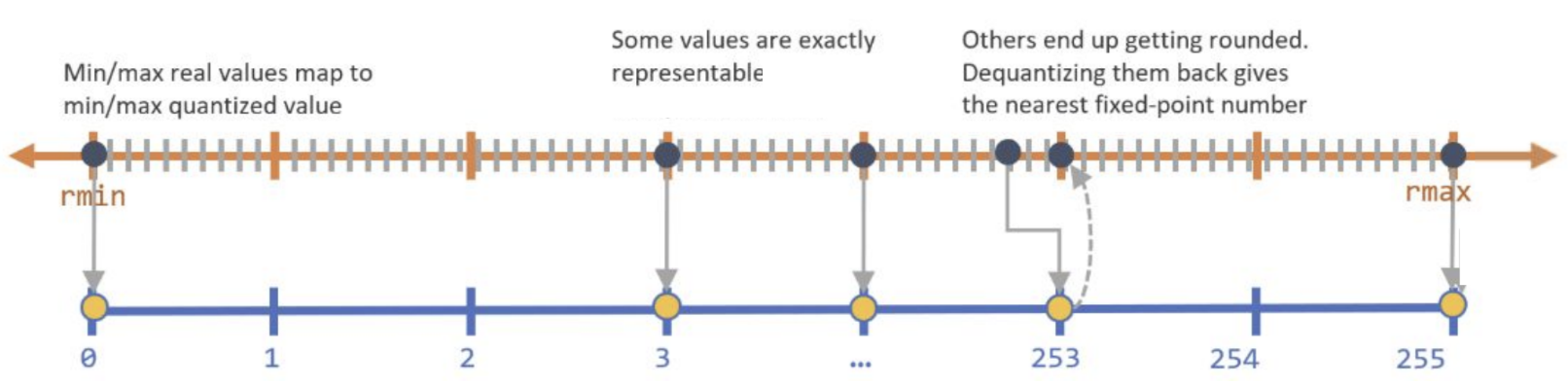
So, how might a mapping between different precisions (i.e. a quantization scheme) work? In a neural network, the weights or activation outputs of a particular layer tend to be normally distributed within a certain range, so ideally a quantization schema takes advantage of this fact and adapts to fit each layer’s individual distribution. For example, models weights are typically stored as 32-bit floating point numbers and a common approach is to reduce these to 8-bit fixed points (though some techniques have even gone as far as to represent them with single bits!), for which there are 2⁸ = 256 possible values: in the simplest case, we can take the min and max weights of a layer, divide the range between the two into 255 evenly-spaced intervals, and bin the weights according to the interval edge they are closest to:
那么,不同精度之间的映射(即量化方案 )如何工作? 在神经网络中,特定层的权重或激活输出倾向于正态分布在某个范围内,因此理想情况下,量化方案可以利用这一事实,并适应每个层的单独分布。 例如,模型权重通常存储为32位浮点数,一种常见的方法是将其减少为8位固定点(尽管有些技术甚至可以用单个位来表示它们!),为此有2个= 256个可能的值:在最简单的情况下,我们可以取一层的最小和最大权重,将两者之间的范围划分为255个均匀间隔的间隔,并根据距离最接近的间隔边对权重进行分箱至:
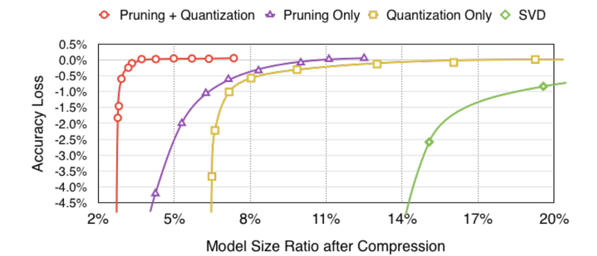
We can see how quantizing the weights in this way would reduce their memory footprint by 4x. And there are many other, more complex techniques that achieve lower information loss, such as an implementation by Han et. al that involves k-means clustering. Specifically, their compression pipeline combines weight pruning, quantization, and Huffman coding, and we can see in the following graph how pruning and quantization of AlexNet trained on ImageNet work together to achieve a model that is 3.7% of its original size with no loss in accuracy:
我们可以看到以这种方式量化权重将如何减少其内存占用量4倍。 还有许多其他更复杂的技术可以降低信息丢失,例如Han等人的实现 。 所有涉及k均值聚类的算法。 具体来说,他们的压缩流水线结合了权重修剪,量化和霍夫曼编码 ,在下图中,我们可以看到在ImageNet上训练的AlexNet的修剪和量化如何协同工作,以实现其原始大小的3.7%的模型而不会造成任何损失。准确性:
In addition to weights, neural networks also consist of operators such as matrix multiplication, convolution, activation functions and pooling that must also be quantized to deal with lower precision weights. While the general idea is the same, quantizing operators is a bit trickier than quantizing pre-trained weights because they have to deal with potential bit overflows and unseen inputs, which can make determining a schema difficult. Luckily, many deep learning softwares, such as TensorFlow, PyTorch, and MXNet, have functionality for quantizing commonly-used operators (if you’re interested, this blog provides high level explanation of TensorFlow’s process), which can yield networks with significantly diminished latency given the increased efficiency of lower precision operations.
除权重外,神经网络还包含诸如矩阵乘法,卷积,激活函数和池化之类的运算符,必须对这些运算符进行量化以处理较低精度的权重。 尽管总体思路是相同的,但量化运算符比量化预训练的权重要复杂一些,因为它们必须处理潜在的位溢出和看不见的输入,这可能会使确定方案变得困难。 幸运的是,许多深度学习软件(例如TensorFlow , PyTorch和MXNet )具有量化常用运算符的功能(如果您有兴趣, 此博客提供了TensorFlow流程的高级解释),可以产生延迟显着减少的网络鉴于低精度操作的效率提高了。
In practice, quantization can be difficult to actually implement because it requires having a decent understanding of hardware and bit-wise computations. It turns out that deciding upon the degree of precision to compress a model to is not as simple as picking a random number of bits: you have to make sure the hardware you’re using is even capable of handling numbers of that size, let alone of doing so efficiently. In reviewing the literature, I found that the savings offered by many state-of-the-art quantization implementations are tied to the features of the hardware being used, although here exist other means of compression that generalize well across many kinds of hardware, such as low-rank factorization.
在实践中,量化可能很难实际实现,因为它需要对硬件和逐位计算有一个体面的了解。 事实证明,决定将模型压缩到的精度并不像选择随机数那么简单:您必须确保所使用的硬件甚至能够处理该大小的数字,更不用说了如此高效地进行。 在查阅文献时,我发现许多最新的量化实现所提供的节省都与所使用硬件的功能有关,尽管这里存在其他压缩方式,可以很好地推广到多种硬件上,例如作为低阶分解。
低阶近似 (Low-rank approximation)
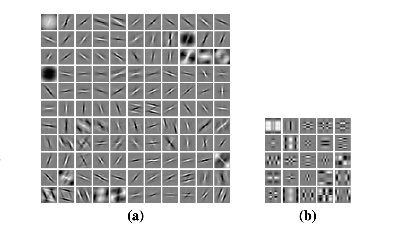
We’re aware that deep neural networks tend to be over-parametrized, with a lot of similarity—or redundancy—occurring between different layers and/or channels. For example, image a above shows filters of a convolutional layer learned for an image segmentation task, many of which look nearly the same. The goal of low-rank approximation is to approximate the numerous, redundant filters of a layer using a linear combination of fewer filters, such as those represented in image b. Compressing layers in this way reduces the network’s memory footprint as well as the computational complexity of convolutional operations and can yield significant speedups.
我们知道,深度神经网络往往被过度参数化, 在不同层和/或通道之间会出现很多相似性或冗余性。 例如,上面的图像a显示了为图像分割任务而学习的卷积层过滤器,其中许多看起来几乎相同。 低秩逼近的目标是使用更少的滤波器(如图像b中表示的滤波器)的线性组合来逼近一层的大量冗余滤波器。 以这种方式压缩层减少了网络的内存占用以及卷积运算的计算复杂度,并可以显着提高速度。
Specifically, the filters in b are of lower rank than those in a. The rank of a matrix is defined as the dimension of the vector space spanned by its columns, which is equal to its number of linearly-independent columns. To illustrate, say we have the following matrix:
具体而言,在b中的过滤器比那些在较低级的。 矩阵的秩定义为由其列跨越的向量空间的维,该维等于其线性独立列的数量。 为了说明,假设我们有以下矩阵:
[[1, 0, -1],
[-2, -3, 1],
[3, 3, 0]]
If we look at just the first two columns, we see that they are linearly independent because neither can be computed from the other using linear operations, so the matrix has to have a rank of at least 2. But if we look at all three columns, we see that if we subtract the first from the second, we get the third, thus all three are not linearly independent and the matrix only has a rank of 2.
如果只看前两列,我们会发现它们是线性独立的,因为两者都不能使用线性运算来计算,因此矩阵的秩必须至少为2。但是如果我们看全部三列,我们看到如果从第二个减去第一个,我们得到第三个,因此所有三个都不是线性独立的,矩阵的秩仅为2。
Intuitively, we get the sense that if an element of a matrix can be computed using others that are present, there is some redundancy of information occurring in the matrix. While individual filters and channels in a network tend to be full rank, indicating no redundancy within themselves, there is typically significant redundancy between different filters or channels. And since low-rank matrices encode redundant information, it makes sense that we can use them to approximate these redundant layers of a network, which is exactly what low-rank approximation does. To understand the intuition behind how this might be achieved, let’s take a look at a relatively simple approach from Jaderberg et al. that takes advantage of cross-filter redundancy.
从直觉上讲,我们可以感觉到,如果可以使用存在的其他元素来计算矩阵的元素,则矩阵中会出现一些冗余信息。 而在网络中的各个滤波器与信道往往是满秩,这表明自身内没有冗余,典型地存在不同的滤波器或信道之间的显著冗余。 而且由于低秩矩阵对冗余信息进行了编码,因此我们可以使用它们来近似网络的这些冗余层,这很有意义,这正是低秩近似所做的。 为了了解如何实现此目标的直觉,让我们看一下Jaderberg等人的一种相对简单的方法。 利用交叉过滤器冗余。
The following represents a convolution operation with N 2D filters, W, on a single channel feature map, Z, to output an N-channel feature map.
下图表示在单通道特征图Z上使用N个2D滤波器W进行卷积运算以输出N通道特征图。
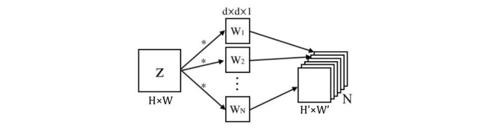
The goal is to reduce the computational complexity of these operations by approximating the N full rank filters with a linear combination of M lower rank filters where M<N, based on the assumption that there is redundancy between the N filters. Specifically, Jadenberg et al. impose that the new filters be of rank 1. If a matrix has rank 1, it means that if we select one of its columns, all the other columns will be some multiple of that column. Thus, rank 1 matrices can be factorized or decomposed to be products of a column vector and a row vector—a property called separability—for example:
目的是基于N个滤波器之间存在冗余的假设,通过用M个低秩滤波器的线性组合近似M个N个低秩滤波器来近似化N个满秩滤波器,从而降低这些运算的计算复杂度。 具体来说,Jadenberg等。 强制新过滤器的等级为1。如果矩阵的等级为1,则意味着如果我们选择其一列,则所有其他列将是该列的倍数。 因此,可以将1级矩阵分解或分解为列向量和行向量的乘积(这种性质称为可分离性) ,例如:
[[1, 4, 5],          [[1],   [[1, 4, 5]]
[2, 8, 10],     =     [2], *
[3, 12, 15]]          [3]]
By imposing separability of the M basis filters and adding a layer to approximate the N output channels of the original convolution operation from the compressed basis, we arrive at a transformed operation that looks like this:
通过强加M个基本滤波器的可分离性,并从压缩的基础上增加一个层来近似原始卷积运算的N个输出通道,我们得到一个转换后的运算,如下所示:

While it may look more complex, it is actually a more computationally efficient operation if M is made to be sufficiently small. The separable bases for these modified layers are optimized asynchronously by minimizing the reconstruction error between the output of the original layer and the output of the approximation layer. Jaderberg et al. use a similar approach to exploit redundancy between channels, with which they achieve 4.5× speedup of a shallow network trained for a text classification task with only a 1% drop in classification accuracy.
尽管看起来可能更复杂,但是如果将M设置得足够小,实际上是一种计算效率更高的操作。 通过最小化原始层的输出与近似层的输出之间的重构误差,可以异步优化这些修改层的可分离基础。 Jaderberg等。 使用类似的方法来利用通道之间的冗余,通过这种方法,他们可以使为文本分类任务训练的浅层网络的速度提高4.5倍,而分类准确率仅下降1%。
If you take a look at the literature on low-rank approximation, it’s likely you’ll come across the terms SVD (“Singular Value Decomposition”), Tucker decomposition and CP (“Canonical Polyadic”) decomposition, so it bears briefly explaining the designation between these. SVD stands for “Singular Value Decomposition” and is a matrix factorization. In the context of approximating a matrix M with another matrix M’ of a lower rank r as we’ve discussed, the optimal M’ is equal to the SVD of M constrained by r. Tucker and CP decomposition are ways of generalizing SVD to tensors. As you likely know, a tensor is a multi-dimensional array. Tucker decomposition decomposes a tensor into a set of matrices and one small core tensor. CP is actually a special case of Tucker decomposition that decomposes a tensor into a sum of rank-1 tensors, though they are often referred to in the literature as two separate approaches. We can see how they both work in 3D space below:
如果您查看有关低秩逼近的文献,则可能会遇到SVD(“奇异值分解”),Tucker分解和CP(“规范多阿迪克”)分解这两个词,因此它需要简要说明这些之间的名称。 SVD代表“奇异值分解”,是矩阵分解。 在近似矩阵M与另一矩阵M的上下文“因为我们已经讨论较低秩r的,最佳的M”是等于M的SVD约束用r。 Tucker和CP分解是将SVD泛化为张量的方法 。 如您所知,张量是多维数组。 Tucker分解将张量分解为一组矩阵和一个小的核心张量。 CP实际上是Tucker分解的一种特殊情况,它将张量分解为1级张量之和,尽管在文献中通常将它们称为两种单独的方法。 我们可以在下面的3D空间中看到它们的工作原理:

Both have their benefits and drawbacks, which you can read more about here, and are popular approaches to low-rank approximation of deep neural networks. Kim et al., for example, achieve substantial compression using Tucker decomposition. They take a data-driven approach to determining the ranks that the compressed layers should have and then perform Tucker decomposition according to these ranks. They apply this compression to various models for image classification tasks and run them on both a Titan X and Samsung Galaxy S6 smartphone, which, notably, has a GPU with 35× lower computing ability and 13× smaller memory bandwidth than Titan X. The following table shows the compressed models’ drops in performance and reductions in size and FLOPs from the original, as well as their time and energy consumption to process a single image.
两者都有其优点和缺点,您可以在此处详细了解,它们都是深层神经网络的低秩逼近的流行方法。 Kim等。 例如,使用Tucker分解实现实质压缩。 他们采用数据驱动的方法确定压缩层应具有的等级,然后根据这些等级执行Tucker分解。 他们将此压缩应用于各种模型以执行图像分类任务,并在Titan X和Samsung Galaxy S6智能手机上运行它们,特别是,其GPU的计算能力比Titan X低35倍,内存带宽比Titan X小13倍。下表显示了压缩模型的性能下降,尺寸和原始尺寸的减少,以及处理单个图像的时间和能耗。

With these results, Kim et al. demonstrate that low-rank approximation is an effective means of compression to achieve significant size and latency reductions in deep neural networks for their potential deployment on mobile devices. And as I mentioned before, a large upside to low-rank approximation as a compression technique is that, since it simplifies model structure just by reducing parameter count, it does not require specialized hardware to implement.
有了这些结果,金等。 演示了低秩逼近是有效压缩的一种有效方法,可实现深度神经网络在移动设备上的潜在部署,从而显着减小大小和延迟。 正如我之前提到的,作为压缩技术,低秩近似的一大优势在于,由于仅通过减少参数数量即可简化模型结构,因此无需专用硬件即可实现。
知识升华 (Knowledge distillation)
If we think about it, the need to compress neural networks arises from the fact that training and inference are two fundamentally different tasks. During training, for example, a model does not have to operate in real time and does not necessarily face restrictions on computational resources, as its primary goal is simply to extract as much structure from the given data as possible, but latency and resource consumption do become of concern if it is to be deployed for inference. As a result, trained models are often larger and slower than what would be ideal for inference and, hence, we have to develop ways compress them. To address this problem, Cornell researchers proposed in 2006 the idea of transferring the knowledge from a large trained model (or ensemble of models) to a smaller model for deployment by training it to mimic the larger model’s output, a process that Hinton et al. generalized in 2014 and gave the name distillation. In short, knowledge distillation is motivated by the idea that training and inference are different tasks such that a different model should be used for each.
如果我们考虑一下,压缩神经网络的需求就来自这样一个事实,即训练和推理是两个根本不同的任务。 例如,在训练过程中,模型不必实时运行,也不必面对计算资源的限制,因为其主要目标只是从给定数据中提取尽可能多的结构,但是延迟和资源消耗确实可以做到。如果要将其部署以进行推理,则会引起关注。 结果,经过训练的模型通常比推理的理想模型更大且更慢,因此,我们必须开发压缩模型的方法。 为了解决这个问题,康奈尔大学的研究人员在2006年提出了一种想法,即通过训练知识以模仿较大模型的输出,将知识从大型训练模型(或模型集合)转移到较小模型以进行部署,这一过程由Hinton等人完成。 于2014年通用 ,并命名为蒸馏 。 简而言之,知识的提炼是由这样的思想激发的,即训练和推理是不同的任务,因此每个模型都应使用不同的模型。

In Hinton et al.’s implementation, the small “student” network learns to mimic the large “teacher” network by minimizing a loss function in which the target is based on the distribution of class probabilities outputted by the teacher’s softmax function. To understand this, let’s review how the softmax function works: it takes in a a logit for a particular class, z_i, and converts it to a probability by dividing it by the sum of logits of all j classes:
在Hinton等人的实现中,小型“学生”网络通过最小化损失函数来学习模仿大型“教师”网络,在该函数中,目标基于教师的softmax函数输出的课堂概率分布。 为了理解这一点,让我们回顾一下softmax函数的工作原理:它获取特定类z_i的一个logit,并将其除以所有j个类的logit的总和,从而将其转换为概率:

Here, the term T is the temperature, of which higher values correspond to “softer” outputs. T is usually set to 1, which results in “hard” outputs in which the correct class label is assigned a probability close to 1, indicating near certainty in this prediction, while the others are assigned probabilities close to 0. Hinton et al. suggest, however, that the distribution of the incorrect class labels holds valuable information about the data that can to be learned from, as they describe in the context of a handwritten digit classification task:
在此,术语T是温度,其较高的值对应于“较软”的输出。 T通常设置为1,这会导致“硬”输出,其中为正确的类别标签分配的概率接近1,表明此预测接近确定,而其他输出的概率分配为接近0。Hinton等。 但是,建议在不正确的类别标签的分发中包含有关可以从中学习的数据的有价值的信息,正如它们在手写数字分类任务的上下文中所描述的:
“One version of a 2 may be given a probability of 10^-6 of being a 3 and 10^−9 of being a 7 whereas for another version it may be the other way around. This is valuable information that defines a rich similarity structure over the data (i. e. it says which 2’s look like 3’s and which look like 7’s)…”
“ 2的一个版本可能被赋予10 ^ -6为3的概率,而10 ^ -9则为7的概率,而对于另一版本,则可能是相反的情况。 这是有价值的信息,它定义了数据上的丰富相似性结构(即,它说哪个2看上去像3一样,哪个看上去像7一样……)”
To capitalize upon this information, Hinton et al. raise the temperature T in the teacher network’s softmax function to soften the distribution of probabilities over the class labels in a process they call distillation, as demonstrated in the following:
为了利用此信息,Hinton等人(2003年)。 在教师网络的softmax函数中提高温度T ,以在他们称为蒸馏的过程中软化类标签上的概率分布,如下所示:

The student network is then trained to minimize the sum of two different cross entropy functions: one involving the original hard targets obtained using a softmax with T=1 and one involving the softened targets. Hinton et al. demonstrate the effectiveness of this technique by training a teacher network with two hidden layers of 12,000 units and a student with two hidden layers of only 800 units. On a test set, the teacher achieves 67 test errors and the student achieves 74, as compared to the 146 test errors made by a network of the same size as the student but that was trained without distillation.
然后训练学生网络以最小化两个不同的交叉熵函数之和:一个涉及使用T = 1的softmax获得的原始硬目标,另一个涉及软化目标。 Hinton等。 通过培训一个具有两个12,000个单位的隐藏层的教师网络和一个具有800个单位的两个隐藏层的学生来演示此技术的有效性。 在测试集上,与通过与学生相同规模但未经蒸馏训练的网络进行的146次测试错误相比,教师达到67次测试错误,而学生达到74次。
After this initial breakthrough by Hinton et al. of training the student to imitate the softmax outputs of a teacher, researchers Romero et al. found that the student can also use information from the teacher’s intermediate hidden layers to improve its final performance. Specifically, they propose what they call “FitNets,” which are student networks that are thinner but deeper than their teachers, with their increased depth allowing them to generalize well while their small widths still make them compact. Romero et al. introduce one “guided layer” in the middle of the student network that is tasked with learning from one “hint” layer in the middle of the teacher network. The table below demonstrates the speedup, reduced parameter count, and generally increased accuracy the FitNets of varying sizes achieve as compared to their teacher architecture on the CIFAR-10 image classification dataset. Further, their performance was on-par with state-of-the-art methods, of which the highest accuracy at the time was 91.78%:
经过Hinton等人的初步突破。 研究人员Romero等人训练学生模仿老师的softmax输出。 发现学生还可以使用教师中间隐藏层中的信息来提高其最终表现。 具体来说,他们提出了所谓的“ FitNets”,即比教师更薄但更深的学生网络,随着深度的增加,他们可以很好地泛化,而较小的宽度仍使它们紧凑。 罗梅罗等。 在学生网络中间引入一个“引导层”,其任务是从教师网络中间的一个“提示”层中学习。 下表展示了与CIFAR-10图像分类数据集上的教师体系结构相比,各种尺寸的FitNet所能实现的加速,减少的参数数量以及通常提高的准确性。 此外,它们的性能可与最新方法媲美,其中当时的最高准确性为91.78%:

Impressive results like these have spurred research on a wide range of different methods for transferring knowledge from teacher to student networks. Indeed, the field of research on knowledge distillation has become so broad and specialized in some areas that it is difficult to evaluate the overall efficacy of general approaches against one another. A drawback of knowledge distillation as a compression technique, therefore, is that there are many decisions that must be made up-front by the user to implement it; for example, unlike the other compression techniques we’ve discussed, the compressed network doesn’t even need to have a similar structure to the original. But this also means that knowledge distillation is very flexible and can be adapted to a wide range of tasks. If you’re interested in learning more about different knowledge distillation techniques, this 2020 paper performs a comprehensive review of state-of-the-art approaches for vision-based tasks.
像这样令人印象深刻的结果刺激了人们对将知识从教师网络转移到学生网络的各种不同方法的研究。 确实,关于知识蒸馏的研究领域已经变得如此广泛和专门,以致于某些领域难以相互评价通用方法的整体功效。 因此,知识蒸馏作为一种压缩技术的一个缺点是,用户必须预先做出许多决定才能实施它。 例如,与我们讨论过的其他压缩技术不同,压缩网络甚至不需要具有与原始网络类似的结构。 但这也意味着知识提炼非常灵活,可以适应各种各样的任务。 如果您想了解更多有关不同知识提炼技术的知识, 本2020年的论文将对基于视觉的任务的最新方法进行全面回顾。
神经架构搜索(NAS) (Neural Architecture Search (NAS))
The reality is that multiple of the compression techniques we’ve discussed so far could be applied in a given scenario, and when you take into account combinations of them, the number of possible architectures to explore expands dramatically. The hard part is, of course, choosing the optimal one. This is where Neural Architecture Search (NAS) comes in. NAS in the most general sense is a search over a set of decisions that define the different components of a neural network—it is a systematic, automized way of learning optimal model architectures. The idea is to remove human bias from the process to arrive at novel architectures that perform better than human-designed ones.
现实情况是,到目前为止,我们已经讨论了多种压缩技术,可以在给定场景中使用它们,并且当您考虑到它们的组合时,可以探索的可能架构的数量会急剧增加。 当然,最困难的部分是选择最佳的。 这就是神经体系结构搜索(NAS)出现的地方。从最一般的意义上讲,NAS是对一组定义神经网络的不同组成部分的决策进行的搜索-这是学习最佳模型体系结构的系统化,自动化方法。 这样做的目的是消除流程中的人为偏差,从而得出性能优于人为设计的新颖架构。
Obviously, for any given task there are infinite possible model architectures to explore and, with this, many different approaches to searching through them. A 2019 survey categorizes different NAS techniques according to the following three dimensions:
显然,对于任何给定的任务,都有无限可能的模型架构可供探索,并且由此可以找到许多不同的搜索方法。 2019年的一项调查根据以下三个维度对不同的NAS技术进行了分类:
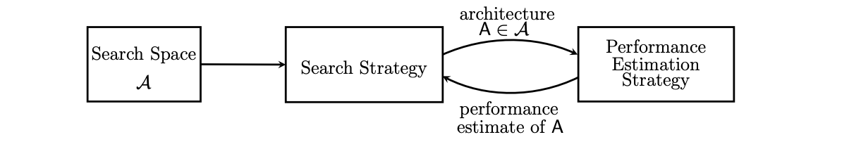
Search space: The possible architectures that can be discovered in the search. We’re aware that networks can consist of a whole host of operations such as convolutions, pooling, concatenation and activation functions, and defining a search space involves imposing constraints on how and which of these components can be combined to generate the networks that are searched through. For example, defining a search space might involve restricting the number of possible convolutional layers the network can have or requiring it to repeat a general pattern of operations several times. Inevitably, imposing such restrictions introduces some human bias into the search process. And even with these restrictions, the search space will still be very large, as is the point of NAS — to discover and evaluate architectures outside of the realm of what we might normally construct.
搜索空间 :可以在搜索中发现的可能架构。 我们知道,网络可以包括卷积,池化,串联和激活函数之类的全部操作,并且定义搜索空间涉及对如何以及如何组合这些组件来生成要搜索的网络施加约束。通过。 例如,定义搜索空间可能涉及限制网络可能具有的可能卷积层的数量,或者要求其重复几次常规操作模式。 不可避免地,施加这样的限制会在搜索过程中引入一些人为的偏见。 即使有这些限制,NAS的要点仍然是很大的搜索空间-在我们通常可能构建的领域之外发现和评估架构。
Search strategy: The strategy followed to guide the exploration of the search space, i.e. what determines the next architectures to explore in the search. While this could be random, it’s unlikely given the huge scope of a given search space that an optimal architecture will be happened upon by random chance, so the search strategy typically takes into account the performance of previously explored architectures. For example, so-called “evolutionary” algorithms are based on maintaining an evolving population of candidate architectures throughout the training process. There are also reinforcement-learning-based strategies where an agent is trained to estimate the performance of architectures on unseen data.
搜索策略 :遵循该策略来指导搜索空间的探索,即决定下一个要在搜索中探索的体系结构的因素。 尽管这可能是随机的,但鉴于给定搜索空间的范围之大,不太可能偶然出现最佳架构,因此搜索策略通常会考虑以前探索过的架构的性能。 例如,所谓的“进化”算法是基于在整个训练过程中保持不断发展的候选体系结构。 还有一些基于强化学习的策略,在这些策略中,对代理进行了培训,以根据看不见的数据估计体系结构的性能。
Performance estimation strategy: How the performance of candidate models on unseen data is estimated. Performance feedback is used to optimize the search strategy. This can be as simple as training each network from scratch and measuring their accuracy on a validation set, but this can be very costly; thus, strategies that involve parameter sharing between many models or that use low-fidelity approximations of data or the networks themselves, for example, have been developed.
绩效评估策略 :如何评估候选模型在看不见的数据上的绩效。 性能反馈用于优化搜索策略。 这很简单,例如从头开始训练每个网络并在验证集上测量其准确性,但这可能会非常昂贵。 因此,例如,已经开发出涉及在许多模型之间进行参数共享或者使用数据或网络本身的低逼真度近似的策略。
As you can imagine, NAS is a very broad field of research, so here we will just focus on its use for compressing pre-trained models, specifically. In 2018, for example, He et al. introduced AutoML for Model Compression (AMC), a technique that uses a reinforcement learning search strategy to compress pre-trained networks layer-by-layer. Specifically, AMC’s search space is parametrized by a user-defined, hardware-based constraint such as maximum latency, model size, or number of FLOPS. The agent proceeds through the network one layer at a time, outputting a compression ratio that is based on the composition of the layer and that also adheres to the hardware constraint. After all layers are pruned according to their ratios via a structured or unstructured approach, the validation accuracy of the compressed model is computed without fine-tuning and used as the agent’s reward. Forgoing fine-tuning after compressing the model is a tactic He et al. take in their performance estimation strategy that allows for faster policy exploration.
As you can imagine, NAS is a very broad field of research, so here we will just focus on its use for compressing pre-trained models, specifically. In 2018, for example, He et al. introduced AutoML for Model Compression (AMC), a technique that uses a reinforcement learning search strategy to compress pre-trained networks layer-by-layer. Specifically, AMC's search space is parametrized by a user-defined, hardware-based constraint such as maximum latency, model size, or number of FLOPS. The agent proceeds through the network one layer at a time, outputting a compression ratio that is based on the composition of the layer and that also adheres to the hardware constraint. After all layers are pruned according to their ratios via a structured or unstructured approach, the validation accuracy of the compressed model is computed without fine-tuning and used as the agent's reward. Forgoing fine-tuning after compressing the model is a tactic He et al. take in their performance estimation strategy that allows for faster policy exploration.
AMC’s learning-based pruning was tested against handcrafted, rule-based approaches on various models and was found to exhibit all-around superior performance. For example, the following table shows the results of AMC’s compression with a 50% FLOP or 50% latency constraint on MobileNet as compared to a rule-based strategy that prunes the network to 75% of its original parameters (second row):
AMC's learning-based pruning was tested against handcrafted, rule-based approaches on various models and was found to exhibit all-around superior performance. For example, the following table shows the results of AMC's compression with a 50% FLOP or 50% latency constraint on MobileNet as compared to a rule-based strategy that prunes the network to 75% of its original parameters (second row):

As we can see, the networks pruned with AMC achieve nearly the same accuracy as the original MobileNet (top row) with reduced latency and memory size, as opposed to the rule-based pruning technique.
As we can see, the networks pruned with AMC achieve nearly the same accuracy as the original MobileNet (top row) with reduced latency and memory size, as opposed to the rule-based pruning technique.
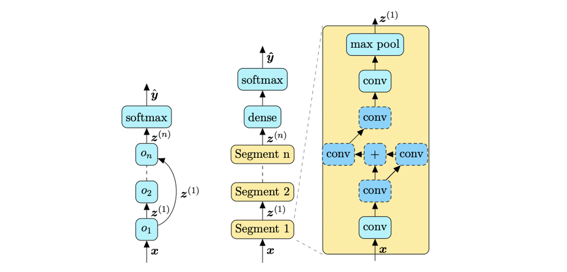
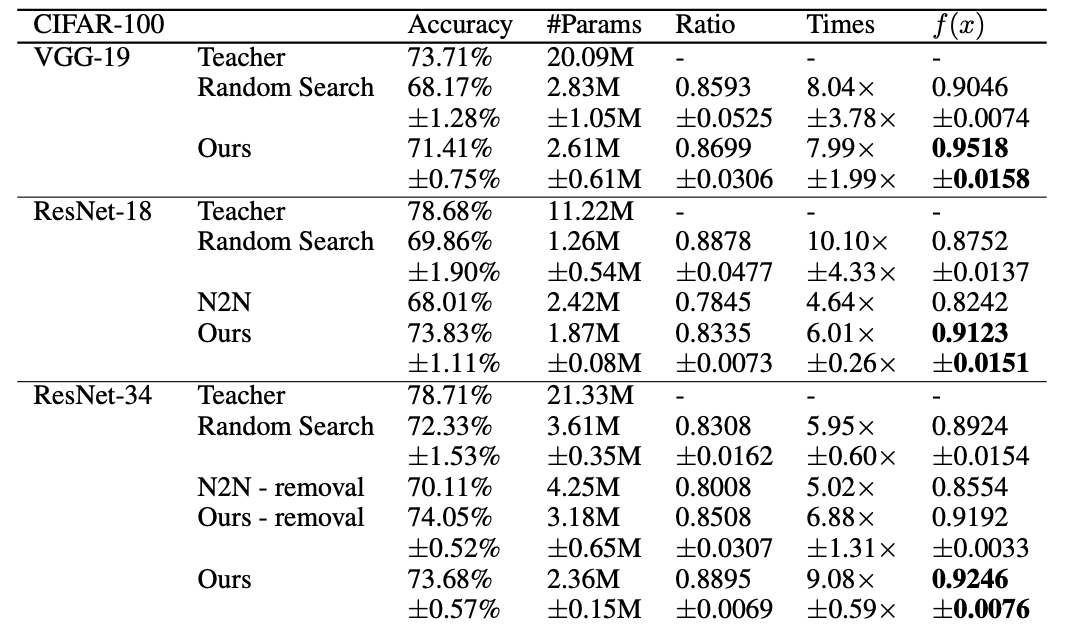
More recently in 2019, Cao et al. use Bayesian Optimization to search for an optimal compressed architecture. In their implementation, they continuously add to a set models that are all based on an original network but have been compressed by randomly removing or shrinking layers and adding skip connections. These architectures are evaluated based on the reduced parameter count and accuracy they achieve as compared to the original. Over a number of epochs, the models are sampled from and used to learn to predict to what extent new, randomly generated compressed models will outperform the current best model of the set in terms of compression and accuracy—this way, the randomly generated architectures don’t have to go through the time-intensive process of actually be evaluated on data and more architectures can be explored instead. Based on these predictions, the most promising of the newly generated models are evaluated on data and added to the growing set of models, and the process continues. At the end, the best model of the set in terms of compression and accuracy is selected. The following table demonstrates the effectiveness of Cao et al.’s approach on compressing three architectures for image classification on the CIFAR-100 dataset as compared to a random NAS approach and to Ashok et. al’s state-of-the-art “N2N” technique.
More recently in 2019, Cao et al. use Bayesian Optimization to search for an optimal compressed architecture. In their implementation, they continuously add to a set models that are all based on an original network but have been compressed by randomly removing or shrinking layers and adding skip connections. These architectures are evaluated based on the reduced parameter count and accuracy they achieve as compared to the original. Over a number of epochs, the models are sampled from and used to learn to predict to what extent new, randomly generated compressed models will outperform the current best model of the set in terms of compression and accuracy—this way, the randomly generated architectures don't have to go through the time-intensive process of actually be evaluated on data and more architectures can be explored instead. Based on these predictions, the most promising of the newly generated models are evaluated on data and added to the growing set of models, and the process continues. At the end, the best model of the set in terms of compression and accuracy is selected. The following table demonstrates the effectiveness of Cao et al.'s approach on compressing three architectures for image classification on the CIFAR-100 dataset as compared to a random NAS approach and to Ashok et. al's state-of-the-art “N2N” technique.
We’ve seen two demonstrations of NAS’s effectiveness at achieving more compact models. The possibilities really are endless with NAS, but successful implementation relies on picking a search space, search strategy, and performance estimation strategy that are suited to the problem at hand, which can require a decent amount of domain knowledge and poses a barrier to entry to it as a compression technique.
We've seen two demonstrations of NAS's effectiveness at achieving more compact models. The possibilities really are endless with NAS, but successful implementation relies on picking a search space, search strategy, and performance estimation strategy that are suited to the problem at hand, which can require a decent amount of domain knowledge and poses a barrier to entry to it as a compression technique.

Luckily, software does exist that abstracts away some of the complexity to make NAS more accessible. For example, Google’s Cloud AutoML makes the process as simple as inputting a training dataset and letting its algorithm search for an optimal set of building blocks for the network—a baseline architecture that the user can fine-tune to optimize further. All of this is done within its GUI to make the process accessible even to inexperienced programmers. Auto-Keras is an open-source NAS package that takes a different approach in that the user specifies the high-level architecture of the model and its algorithm conducts a search through the details of the configuration.
Luckily, software does exist that abstracts away some of the complexity to make NAS more accessible. For example, Google's Cloud AutoML makes the process as simple as inputting a training dataset and letting its algorithm search for an optimal set of building blocks for the network—a baseline architecture that the user can fine-tune to optimize further. All of this is done within its GUI to make the process accessible even to inexperienced programmers. Auto-Keras is an open-source NAS package that takes a different approach in that the user specifies the high-level architecture of the model and its algorithm conducts a search through the details of the configuration.
结论 (Conclusion)
We’ve now developed a basic understanding of the inner workings of a few popular compression techniques for deep learning models. The next step would be to actually try some of them out—a task we’ll tackle in an upcoming blog. Specifically, we’ll use some of the techniques discussed here to compress a few of the winning models from the SpaceNet 6 challenge to demonstrate how networks for building footprint segmentation might be made more resource-efficient for deployment in space.
We've now developed a basic understanding of the inner workings of a few popular compression techniques for deep learning models. The next step would be to actually try some of them out—a task we'll tackle in an upcoming blog. Specifically, we'll use some of the techniques discussed here to compress a few of the winning models from the SpaceNet 6 challenge to demonstrate how networks for building footprint segmentation might be made more resource-efficient for deployment in space.
太空夜景


 37万+
37万+

 被折叠的 条评论
为什么被折叠?
被折叠的 条评论
为什么被折叠?
 到【灌水乐园】发言


