


alexnet vgg
介绍 (Introduction)
In the last article, we reviewed how some of the most famous classification networks are evaluated on ImageNet. We also finished building a PyTorch evaluation dataset class, as well as, efficient evaluation functions. We will soon see how they come handy in validating our model structures and training.
在上一篇文章中 ,我们回顾了如何在ImageNet上评估一些最著名的分类网络。 我们还完成了PyTorch评估数据集类的构建以及高效的评估功能。 我们很快将看到它们如何在验证我们的模型结构和培训时派上用场。
We will build AlexNet and VGG models in this article. Despite their influential contribution to computer vision and deep learning, their structures are straightforward in retrospect. Therefore, in addition to building them, we will also play with “weight porting” and sliding window implementation with convolutional layers.
我们将在本文中构建AlexNet和VGG模型。 尽管它们对计算机视觉和深度学习具有重要影响,但回顾其结构却很简单。 因此,除了构建它们之外,我们还将使用带卷积层的“权重移植”和滑动窗口实现。
I personally find borrowing weights from other models a simple but useful technique to practice. Other than using it to double check our model structure, it can also be used for porting model weights between different frameworks, as well as, initializing the backbone of a detector or a modified network by reshaping the weights (we will dabble in it for our sanity check).
我个人发现从其他模型中借用权重是一种简单但有用的练习方法。 除了使用它来仔细检查我们的模型结构之外,它还可以用于在不同框架之间移植模型权重,以及通过重塑权重来初始化检测器或修改后的网络的主干(我们将涉猎其中)完整性检查)。
Cool, so let’s begin.
太酷了,让我们开始吧。
监督 (Overveiw)
- Explaining the structures of AlexNet and VGG family 解释AlexNet和VGG系列的结构
- Building our own library modules for them 为他们构建我们自己的库模块
- Implementing sliding window with convolution 卷积实现滑动窗口
- Replacing the fully connected classifier head with a convolutional classifier head for “dense evaluation” 用卷积分类器替换完全连接的分类器头以进行“密集评估”
- Discussion on weight initialization 权重初始化的讨论
- Sanity check by porting weights from the pretrained models 通过移植来自预训练模型的权重进行健全性检查
亚历克斯网 (AlexNet)
AlexNet is often regarded as the model that marked the dawn of current deep learning era. It was the winner of ImageNet 2012 with a top 5 accuracy of 15.3%, outperforming the runner-up of the year by a whopping 10.9%.
AlexNet往往被视为标志着当前深度学习时代的到来模型 。 它是ImageNet 2012的赢家,其前5位的准确度为15.3%,比年度亚军高出10.9%。
It has 60 million parameters and given GPUs’ limited memory nearly 10 years ago, AlexNet had to be split and trained across two GTX 580 3GB GPUs. For this reason, it can be confusing to decipher the exact structure of AlexNet for one GPU from the original paper. In fact, the official PyTorch implementation of AlexNet takes reference from this paper (check footnote 1 on page 5), although PyTorch’s implementation still differs from the paper by using 256 kernels in the 4th convolutional layer instead of the 384 described in the paper (aargh!).
它具有6000万个参数,并且在近10年前,由于GPU的内存有限,AlexNet必须在两个GTX 580 3GB GPU上进行拆分和培训。 因此,从原始论文中破译一个GPU的AlexNet的确切结构可能会造成混淆。 实际上,AlexNet的官方PyTorch实现参考了本文 (请参见第5页的脚注1),尽管PyTorch的实现与本文仍然有所不同,在第4卷积层使用了256个内核,而不是论文中描述的384个内核(aargh)。 !)。
We will also ignore the Local Response Normalization (LRN) feature of the network. While the paper states that LRN reduces top1 and top5 by a non-negligible amount (1.4% and 1.2%), it is not often used nowadays as its effects are insignificant for most networks. Batch normalization is the default scheme to apply if we want the model to learn better. We will add that for our VGG networks.
我们还将忽略网络的本地响应规范化(LRN)功能。 尽管该论文指出LRN将top1和top5减少了不可忽略的数量(1.4%和1.2%),但由于它对大多数网络的影响微不足道,因此如今已不常用。 如果我们希望模型学习得更好,则批量标准化是默认的方案。 我们将其添加到我们的VGG网络中。
In this article, we will follow PyTorch’s AlexNet structure so that we can use its pretrained weights. The structure we will use is illustrated in the following figure. The spatial dimension of the feature maps after convolution/max-pooling can be computed as floor(W - F + 2P) / S) + 1where Wis the current feature map’s width/height, Fis the filter’s size, Pis padding size and Sis stride. floor() means we round down to the nearest integer. The “thickness” or “depth” of the output feature maps depend on the number of kernels (filters) we use at current stage.
在本文中,我们将遵循PyTorch的AlexNet结构,以便我们可以使用其预先训练的权重。 下图说明了我们将使用的结构。 卷积/最大合并后的特征图的空间尺寸可以计算为floor(W - F + 2P) / S) + 1 ,其中W是当前特征图的宽度/高度, F是滤镜的大小, P是填充大小和S大步前进。 floor()表示我们舍入到最接近的整数。 输出特征图的“厚度”或“深度”取决于我们在当前阶段使用的内核(过滤器)数量。
With PyTorch library, this AlexNet structure is pretty easy to implement. In the __init__() method, we can first ignore the head argument which controls the what kind of classification head we want to use.
使用PyTorch库,此AlexNet结构非常易于实现。 在__init__()方法中,我们可以首先忽略head参数,该参数控制我们要使用哪种分类head。
As we can see in the code and you may have already known that one beautiful property of convolutional layers is they do not care about your input size. Given any input size, it will generate the corresponding output size according to the formula above. However, if we append the convolutional layers with fully connected layers, then we need to consider the final feature map’s total elements. In AlexNet, the flattened feature map must be a 9216-dimension vector before going into the fully connected classifier.
正如我们在代码中看到的那样,您可能已经知道卷积层的一个美丽属性是它们不关心您的输入大小。 给定任何输入大小,它将根据上面的公式生成相应的输出大小。 但是,如果我们在卷积图层上附加完全连接的图层,则需要考虑最终特征图的全部元素。 在AlexNet中,展平的特征图在进入完全连接的分类器之前必须为9216维向量。
There are two ways to satisfy this constraint. We can either have a resize operation to convert the input images to 224 x 224 dimension, or we can “resize” the final feature to make it 256 x 6 x 6 before put it into the fully connected layers. The second solution can be accomplished with nn.AdaptiveAvgPool2d() . It is kind of analogous to interpolation. A good explanation of it can be found here. With this bit of knowledge, we can build our fully connected classifier.
有两种方法可以满足此约束。 我们可以执行调整大小操作以将输入图像转换为224 x 224尺寸,也可以“调整”最终特征的大小以使其为256 x 6 x 6,然后再放入完全连接的图层中。 第二种解决方案可以使用nn.AdaptiveAvgPool2d()完成。 它有点类似于插值。 可以在这里找到很好的解释。 借助这些知识,我们可以构建完全连接的分类器。
ConvNet的滑动Windows实现 (ConvNet’s Implementation of Sliding Windows)
Fully connected layers are sort of annoying in neural networks for computer vision tasks. It has too much parameters and induces the strict input dimension requirement. So the question is can we do without it? Luckily, yes. In many later networks, fully connected layers are replaced by simple average pooling. In our case, if we want to stay true to the network structure, we can replace it with its equivalent convolutional implementation, ditching the need of ensuring the fixed input size.
在神经网络中,对于计算机视觉任务而言,完全连接的层有点烦人。 它具有太多参数,并引起严格的输入尺寸要求。 因此,问题是我们可以没有它吗? 幸运的是 在许多后来的网络中,完全连接的层被简单的平均池所代替。 在我们的案例中,如果我们希望忠于网络结构,则可以用等效的卷积实现代替它,从而无需确保输入大小固定。
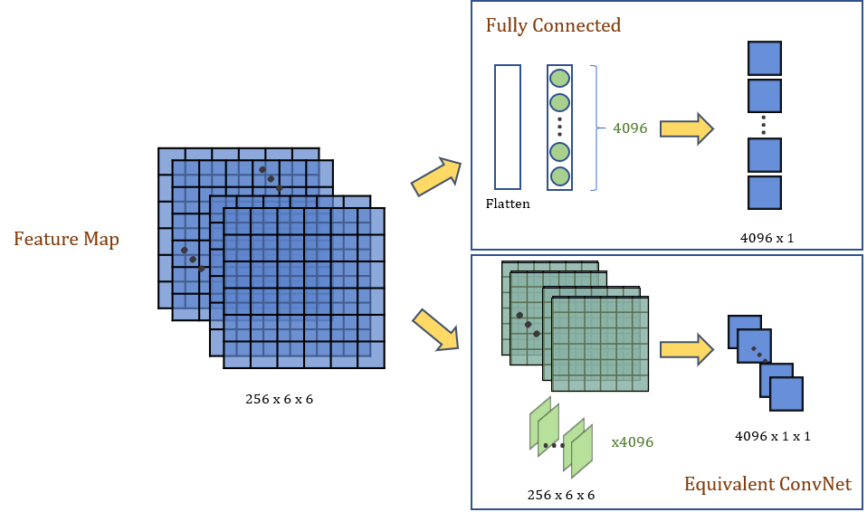
As in the above diagram, the 256 x 6 x 6 final feature map is on the left. It can be flattened to a 9216-dimensional feature vector and passed through a 4096-unit fully connected layer (top right). For every unit (green dot), there are 9216 connections, linking each element on the feature map. It will produce a 4096 x 1 feature vector. In this way, each FC unit is effectively a 256 x 6 x 6 kernel (bottom right). We can thus replace the 4096-unit FC layer with a convolutional layer of 4096 256 x 6 x 6 kernels. It will produce a 4096 x 1 x 1 feature map instead. It is obvious to see that aside from the extra dimension, the two outputs are equivalent.
如上图所示,左侧为256 x 6 x 6最终特征图。 可以将其展平为9216维特征向量,并通过4096个单位的完全连接层(右上)。 对于每个单元(绿色点),都有9216个连接,它们链接特征地图上的每个元素。 它将产生4096 x 1特征向量。 这样,每个FC单元实际上就是256 x 6 x 6内核(右下)。 因此,我们可以用4096 256 x 6 x 6内核的卷积层替换4096个单位的FC层。 它将生成4096 x 1 x 1的特征图。 很明显,除了额外的维度,这两个输出是等效的。
With this derivation, we can implement the ConvNet version of classification head. Continuing from the previous code snippet, we have:
通过此推导,我们可以实现分类头的ConvNet版本。 继续前面的代码片段,我们有:
At the first look, this conversion seems redundant. However, remember the one beautiful property of ConvNet we mentioned minutes ago? Now we can allow the input to have any sizes as long as they are larger than 224 x 224.
乍一看,这种转换似乎是多余的。 但是,还记得我们几分钟前提到的ConvNet的一个美丽属性吗? 现在我们可以允许输入具有任何大小,只要它们大于224 x 224。
For example, if we have an input image with size that is between 287 x 287 and 318 x 318, we will get a final feature map that is 256 x 8 x 8. As our fully connected layers can only take in a flattened feature vector corresponding to a 256 x 6 x 6 feature map, we have to apply nn.AdaptiveAvgPool2d() . Alternatively, we can try “dense evaluation”, that is to put a sliding windows across the feature map and get 9 crops of 256 x 6 x 6 feature map and put them into the FC layers one-by-one to generate final outputs (Figure below, top). The outputs can then be averaged.
例如,如果输入图像的大小在287 x 287和318 x 318之间,则最终的特征图将为256 x 8 x8。因为我们完全连接的图层只能吸收平坦的特征向量对应于256 x 6 x 6特征图,我们必须应用nn.AdaptiveAvgPool2d() 。 另外,我们可以尝试“ 密集评估 ”,即在特征图中放置一个滑动窗口,并获得9个256 x 6 x 6特征图的作物,然后将它们一张一张地放入FC层,以生成最终输出(下图,顶部)。 然后可以平均输出。
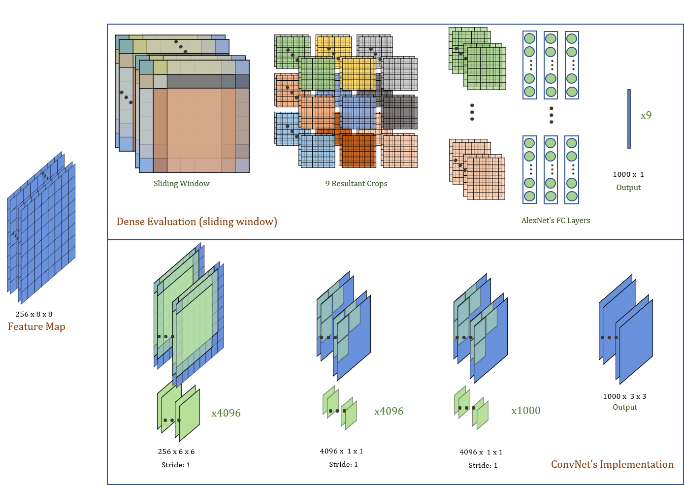
However, if we are using the ConvNet’s implementation of the FC layers, we are naturally using sliding windows (Figure above, bottom). The output feature map can be averaged across the spatial dimension to get the final output.
但是,如果我们使用ConvNet的FC层实现,则自然会使用滑动窗口(上图,底部)。 可以在整个空间维度上对输出要素图进行平均以获得最终输出。
With ConvNet’s implementation of the classification head, we can now be lenient with our input image size.
使用ConvNet实现分类头后,我们现在可以宽容输入图像的大小。
Let’s write the last bit of code to complete our AlexNet implementation. The forward() method of the class is:
让我们写最后的代码来完成我们的AlexNet实现。 该类的forward()方法为:
In the same script, we can define builder function that helps us generate the specified AlexNet. When we have pretrained weights ready, we can load the weights into the network here.
在同一脚本中,我们可以定义构建器函数来帮助我们生成指定的AlexNet。 准备好预训练的权重后,可以在此处将权重加载到网络中。
With that, we have finished our AlexNet model. We can now move on to sanity check with weight porting.
至此,我们完成了AlexNet模型。 现在,我们可以通过重量移植进行健康检查。
重量移植的健全性检查 (Sanity Check with Weight Porting)
We are going to initiate a pretrained AlexNet from torchvision and copy its weight to our model. In this section, we will go through how weights are indexed and how to reshape the weights for our ConvNet implementation of FC classifier.
我们将从火炬视觉中启动经过预训练的AlexNet,并将其权重复制到我们的模型中。 在本节中,我们将介绍如何为FC分类器的ConvNet实现索引权重以及如何调整权重。
Firstly, we initiate all three networks:
首先,我们启动所有三个网络:
Let’s print out all the states and parameters of the three networks. If we run the script at this stage, we should get something like below.
让我们打印出这三个网络的所有状态和参数。 如果我们在此阶段运行脚本,则应获得如下内容。
Torch name: features.0.weight         torch.Size([64, 3, 11, 11])
FC name   : features.0.weight         torch.Size([64, 3, 11, 11])
Conv name : features.0.weight         torch.Size([64, 3, 11, 11])Torch name: features.0.bias           torch.Size([64])
FC name   : features.0.bias           torch.Size([64])
Conv name : features.0.bias           torch.Size([64])Torch name: features.3.weight         torch.Size([192, 64, 5, 5])
FC name   : features.3.weight         torch.Size([192, 64, 5, 5])
Conv name : features.3.weight         torch.Size([192, 64, 5, 5])...Torch name: classifier.0.weight       torch.Size([4096, 25088])
FC name   : classifier.2.weight       torch.Size([4096, 25088])
Conv name : classifier.0.weight       torch.Size([4096, 512, 7, 7])Torch name: classifier.0.bias         torch.Size([4096])
FC name   : classifier.2.bias         torch.Size([4096])
Conv name : classifier.0.bias         torch.Size([4096])Torch name: classifier.3.weight       torch.Size([4096, 4096])
FC name   : classifier.5.weight       torch.Size([4096, 4096])
Conv name : classifier.3.weight       torch.Size([4096, 4096, 1, 1])...
To transfer the weights from PyTorch’s pretrained AlexNet to our AlexNet with FC classification head, we can create an OrderedDict() and store the pretrained AlexNet’s weights with our model’s parameter name. We will then load this OrderedDict to our model.
要将权重从PyTorch的预训练AlexNet转移到带有FC分类头的AlexNet,我们可以创建OrderedDict()并使用模型的参数名称存储预训练的AlexNet的权重。 然后,我们将这个OrderedDict加载到我们的模型中。
This process can be repeated for our AlexNet with Convolutional head. However, as convolutional layers’ weights and FC layers’ weights have different shape, we need to reshape the weights for our classifier.
对于带有卷积头的AlexNet,可以重复此过程。 但是,由于卷积层的权重和FC层的权重具有不同的形状,因此我们需要对分类器的权重进行整形。
During the loading of the weights, there is no error, indicating that we have got the weights’ name and shapes right. However, to guarantee that we have got everything correct, we should test our model with the evaluation script we wrote in the last article.
在加载砝码期间,没有错误,这表明我们正确设置了砝码的名称和形状。 但是,为了确保我们一切都正确,我们应该使用上一篇文章中编写的评估脚本来测试模型。
The torchvision’s pretrained AlexNet and our AlexNet have exactly the same accuracy, indicating we have done everything correctly.
火炬视觉的预训练AlexNet和我们的AlexNet具有完全相同的精度,表明我们已正确完成了所有操作。
Next, let’s conduct the same center-crop evaluation with our convolutionally headed AlexNet. As this AlexNet outputs a feature map instead of a feature vector, we need to first write a wrapper that will average the model’s output.
接下来,让我们与以卷积为首的AlexNet进行相同的中心裁剪评估。 由于此AlexNet输出特征图而不是特征向量,因此我们需要首先编写一个包装程序,以对模型的输出求平均值。
Then, we can pass the wrapped model to our evaluation function to get the outcome.
然后,我们可以将包装的模型传递给评估函数以获取结果。
Finally, we can test the “dense evaluation” by passing images of size larger than 224 x 224 and average the output for prediction.
最后,我们可以通过传递尺寸大于224 x 224的图像并平均输出以进行预测来测试“密集评估”。
As can be seen, the dense evaluation is about 1.3% more accurate than the center-crop evaluation. Yet, because most of the computations from the convolutional feature extractor are shared, the evaluation time isn’t too much longer.
可以看出,稠密评估的准确性比中茬评估高约1.3%。 但是,由于共享了卷积特征提取器的大多数计算,因此评估时间不会太长。
Hooray! now we have our own enhanced AlexNet.
万岁! 现在我们有了自己的增强型AlexNet。
VGG (VGG)
When I first studied neural networks, I felt overwhelmed by the huge combinatorial possibilities of network structure. How deep do I need to go? What would the kernel sizes be? How many kernels should I use? What should the strides be?… AlexNet did not help with my queries. There isn’t too much pattern in the AlexNet that we can follow. Then VGG networks come to rescue!
当我第一次学习神经网络时,我对网络结构的巨大组合可能性感到不知所措。 我需要走多深? 内核大小是多少? 我应该使用几个内核? 大步向前应该是什么?…AlexNet对我的查询没有帮助。 AlexNet中没有太多可遵循的模式。 然后,VGG网络来救援!
VGG family is a landmark in deep learning, not only because it was the runner-up in 2014 ImageNet competition (with an impressive 7.3% top 5 error rate), but it also helped standardise the structure of networks.
VGG系列是深度学习的一个里程碑,不仅因为它是2014年ImageNet竞赛的亚军(前5位错误率高达7.3%),而且还帮助标准化了网络结构。
VGG中的模式 (Patterns in VGG)
Use 3 x 3 convolutional kernels across the network. Two 3 x 3 kernels stacked together have a 5 x 5 receptive field (i.e. one element on its output feature map is derived from a 5 x 5 region on the input image). Three of it stacked together will have a 7 x 7 receptive field. If we use a stack of three 3 x 3 kernels instead of a 7 x7 kernel, not only do we have the same receptive field, we can imbue it with three times more non-linearities (with ReLU), as well as, use a lot less parameters (3x(3x3xCxC) vs 7 x 7 x C x C, assuming the input map and output map both have C channels).
在网络上使用3 x 3卷积内核。 堆叠在一起的两个3 x 3内核具有5 x 5的接收场(即,其输出特征图上的一个元素来自输入图像上的5 x 5区域)。 其中三个堆叠在一起将具有7 x 7的接收场。 如果我们使用三个3 x 3内核而不是7 x7内核的堆栈,那么我们不仅具有相同的接收场,而且还可以使其非线性度提高三倍(使用ReLU),并且使用少得多的参数(假设输入映射和输出映射都具有C通道,则3x(3x3xCxC)与7 x 7 x C x C相比)。
Only use max-pooling of size 2 and stride 2 to downsample feature map. Unlike AlexNet whose some convolutional layers also downsample the feature map, VGG only downsamples the feature map with max-pooling. This means all the convolutional layers have stride 1.
仅使用大小为2和跨度为2的最大合并来对特征图进行下采样。 与AlexNet的一些卷积层也对特征图进行下采样不同,VGG仅使用最大池化对特征图进行下采样。 这意味着所有卷积层的步幅均为1。
Double the channels after every downsampling. As the feature map’s width and height are halved, its channels are doubled with twice as much kernels applied at each convolutional layer.
每次下采样后,将通道加倍。 当特征图的宽度和高度减半时,其通道将加倍,每个卷积层上应用的内核数将增加一倍。
Now we have the luxury of restricted choices while building our networks. In fact, many later networks also adopt these patterns in their structure. We seldom see the use of large kernels nowadays, and the heuristic of only doubling channels after downsampling gives rise to the concept of “module”, a stack of convolutional layers with the same number of kernels.
现在,在建立我们的网络时,我们可以自由选择。 实际上,许多后来的网络在其结构中也采用了这些模式。 如今,我们很少看到使用大内核,并且在降采样后仅将通道加倍的试探法引起了“模块”的概念,即具有相同内核数量的卷积层的堆栈。
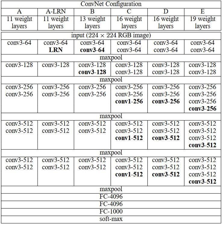
With the above heuristic, the structure of the whole VGG family can be summarized with a single table as in the paper.
通过上述启发式方法,整个VGG系列的结构可以用本文中的单个表格来总结。
With this structured design, we can easily code all the networks in the VGG family.
通过这种结构化设计,我们可以轻松地对VGG系列中的所有网络进行编码。
The code here takes heavy reference of the official code for torchvision’s VGG models. I value-added (hopefully) with detailed remarks.
这里的代码大量引用了Torchvision的VGG模型的官方代码。 我希望通过详细的说明增值。
We first define the structure of the VGG networks. It is basically putting the table above into a dictionary.
我们首先定义VGG网络的结构。 基本上是将上面的表格放入字典中。
Next, we can define the class’s __init__()and forward()methods:
接下来,我们可以定义类的__init__()和forward()方法:
Same as our AlexNet, we will also implement convolutional classification head for VGG (“dense evaluation” originates from VGG paper after all). bn(batch normalization) argument determines if we will include batch normalization into our network. Batch normalization is a technique that came after VGG, we will retrofit it into VGG. It increases both the accuracy and training speed.
与AlexNet一样,我们还将为VGG实现卷积分类头(“密集评估”毕竟源于VGG论文)。 bn (批处理规范化)参数确定是否将批处理规范化包含到我们的网络中。 批量归一化是VGG之后的一项技术,我们将其改装为VGG。 它提高了准确性和训练速度。
We now move onto the _get_conv_layers()method.
现在,我们转到_get_conv_layers()方法。
As mentioned in the comments in the code snippet above, if we choose to add batch normalization, it is usually added after convolution but before non-linearity.
如上面的代码片段中的注释所述,如果我们选择添加批量归一化,则通常在卷积之后但在非线性之前添加。
The classification head’s code is very straightforward too. One thing to note is that dropout, unlike batch normalization, is usually added after activation while before convolution.
分类头的代码也非常简单。 需要注意的一件事是,与批处理规范化不同,通常在激活之后卷积之前添加辍学。
重量初始化 (Weight Initialization)
We are almost done here. However, different from AlexNet whose weights can all be more casually initialized with zero-meaned normal distribution with a standard deviation of 0.01, caution has to be taken in initializing the weights of VGG networks as it is much deeper and does not converge easily. In fact, for ImageNet competition, the authors of VGG first trained shallower versions of the network and then slowly added more layers to make it deeper.
我们在这里差不多完成了。 但是,与AlexNet可以通过零均值正态分布(标准偏差为0.01)更轻松地初始化权重的方法不同,在初始化VGG网络的权重时要格外小心,因为它的深度更深且收敛不容易。 实际上,对于ImageNet竞赛,VGG的作者首先训练了网络的较浅版本,然后慢慢添加了更多层以使其更深。
We do not need to go through that tedious process ourselves, as with Kaiming or Xavier initialization, we can train the whole deep network from scratch. This pdf slides explains the two types of initialization quite well.
我们不需要自己进行繁琐的过程,就像使用Kaiming或Xavier初始化一样,我们可以从头开始训练整个深度网络。 该pdf幻灯片很好地解释了两种类型的初始化。
However, there are a few confusing choices to make. Firstly, for each type of initialization, should we use a Gaussian distribution or uniform distribution? This stackexchange discussion mentions that for Xavier initialization, uniform distribution seems be to slightly better, while for Kaiming initialization, Gaussian distribution is used for all layers in the original ResNet paper, so I guess we can go with Kaiming normal and Xavier uniform distribution.
但是,有一些令人困惑的选择。 首先,对于每种类型的初始化,我们应该使用高斯分布还是均匀分布? 这个stackexchange讨论提到对于Xavier初始化,均匀分布似乎要好一些,而对于Kaiming初始化,高斯分布用于原始ResNet论文中的所有层,因此我想我们可以使用Kaiming正态分布和Xavier均匀分布。
The second question is that for Kaiming initialization, there are “fan-in” and “fan-out” two modes, which one to use? This PyTorch forum discussion states that “fan-in” should be the default mode. It sounds good, except as mentioned in the forum discussion, torchvision’s ResNet as well as VGG used “fan-out”. I did quite a bit of search online but could not find explanation for this choice.
第二个问题是,对于Kaiming初始化,有“扇入”和“扇出”两种模式,该使用哪种模式? 在PyTorch论坛上的讨论指出,“扇入”应为默认模式。 听起来不错,除非在论坛讨论中提到,Torchvision的ResNet以及VGG使用了“扇出”功能。 我在网上做了很多搜索,但是找不到关于此选择的解释。
In this script, I decided to use “fan-in” mode, so the code looks like this:
在此脚本中,我决定使用“扇入”模式,因此代码如下所示:
Just like in AlexNet, we can write some builder functions. Two examples are below:
就像在AlexNet中一样,我们可以编写一些构建器函数。 以下是两个示例:
With this, we completed our implementation of VGG family.
至此,我们完成了VGG系列的实施。
Kudos!
荣誉!
完整性检查 (Sanity Check)
The sanity check for VGG is the same as the one we wrote for AlexNet above. As with AlexNet, “dense evaluation” achieves higher results.
VGG的健全性检查与我们上面为AlexNet编写的检查相同。 与AlexNet一样,“密集评估”可取得更高的结果。
The completed codes for the models can be found in this repository.
可以在此存储库中找到模型的完整代码。
结论 (Conclusion)
In this article, we implemented AlexNet and VGG family. The networks themselves are not difficult to implement, but the idea of using convolutional layers to implement sliding windows, as well as, weight initialization and porting may be tricky to understand.
在本文中,我们实现了AlexNet和VGG系列。 网络本身并不难实现,但是使用卷积层来实现滑动窗口以及权重初始化和端口化的想法可能很难理解。
In the next article, we will write a training script. We will discuss training data augmentation, PyTorch’s data parallelism and distributed data parallelism.
在下一篇文章中,我们将编写一个培训脚本。 我们将讨论训练数据扩充,PyTorch的数据并行性和分布式数据并行性。
翻译自: https://medium.com/swlh/scratch-to-sota-build-famous-classification-nets-2-alexnet-vgg-50a4f55f7f56
alexnet vgg


 3万+
3万+

 被折叠的 条评论
为什么被折叠?
被折叠的 条评论
为什么被折叠?
 到【灌水乐园】发言


