matlab mosaic plot,machinevision-toolbox-matlab

最新推荐文章于 2022-05-15 23:22:48 发布

黄朗文

最新推荐文章于 2022-05-15 23:22:48 发布

阅读量347

点赞数

文章标签： matlab mosaic plot

machinevision-toolbox-matlab.svg?branch=master

Synopsis

Machine Vision Toolbox for MATLAB® release 4.

The Machine Vision Toolbox (MVTB) provides many functions that are useful in machine vision and vision-based control. It is a somewhat eclectic collection reflecting my personal interest in areas of photometry, photogrammetry, colorimetry. It includes over 100 functions spanning operations such as image file reading and writing, acquisition, display, filtering, blob, point and line feature extraction, mathematical morphology, homographies, visual Jacobians, camera calibration and color space conversion. With input from a web camera and output to a robot (not provided) it would be possible to implement a visual servo system entirely in MATLAB.

An image is usually treated as a rectangular array of scalar values representing intensity or perhaps range. The matrix is the natural datatype for MATLAB and thus makes the manipulation of images easily expressible in terms of arithmetic statements in MATLAB language. Many image operations such as thresholding, filtering and statistics can be achieved with existing MATLAB functions.

Advantages of the Toolbox are that:

the code is mature and provides a point of comparison for other implementations of the same algorithms;

the routines are generally written in a straightforward manner which allows for easy understanding, perhaps at the expense of computational efficiency. If you feel strongly about computational efficiency then you can always rewrite the function to be more efficient, compile the M-file using the MATLAB compiler, or create a MEX version;

since source code is available there is a benefit for understanding and teaching.

Code Examples

Binary blobs

>> im = iread('shark2.png'); % read a binary image of two sharks

>> idisp(im); % display it with interactive viewing tool

>> f = iblobs(im, 'class', 1) % find all the white blobs

f =

(1) area=7827, cent=(172.3,156.1), theta=-0.21, b/a=0.585, color=1, label=2, touch=0, parent=1

(2) area=7827, cent=(372.3,356.1), theta=-0.21, b/a=0.585, color=1, label=3, touch=0, parent=1

>> f.plot_box('g') % put a green bounding box on each blob

>> f.plot_centroid('o'); % put a circle+cross on the centroid of each blob

>> f.plot_centroid('x');

Binary blob hierarchy

We can load a binary image with nested objects

>> im = iread('multiblobs.png');

>> idisp(im)

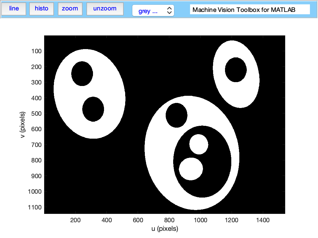
and request the blob label image which we then display

>> [label, m] = ilabel(im);

>> idisp(label, 'colormap', jet, 'bar')

Camera modelling

>> cam = CentralCamera('focal', 0.015, 'pixel', 10e-6, ...

'resolution', [1280 1024], 'centre', [640 512], 'name', 'mycamera')

cam =

name: mycamera [central-perspective]

focal length: 0.015

pixel size: (1e-05, 1e-05)

principal pt: (640, 512)

number pixels: 1280 x 1024

pose: t = (0, 0, 0), RPY/yxz = (0, 0, 0) deg

and its intrinsic parameters are

>> cam.K

ans =

1.0e+03 *

1.5000 0 0.6400

0 1.5000 0.5120

0 0 0.0010

We can define an arbitrary point in the world

>> P = [0.3, 0.4, 3.0]';

and then project it into the camera

>> cam.project(P)

ans =

790

712

which is the corresponding coordinate in pixels. If we shift the camera slightly the image plane coordiante will also change

>> cam.project(P, 'pose', SE3(0.1, 0, 0) )

ans =

740

712

We can define an edge-based cube model and project it into the camera's image plane

>> [X,Y,Z] = mkcube(0.2, 'pose', SE3(0, 0, 1), 'edge');

>> cam.mesh(X, Y, Z);

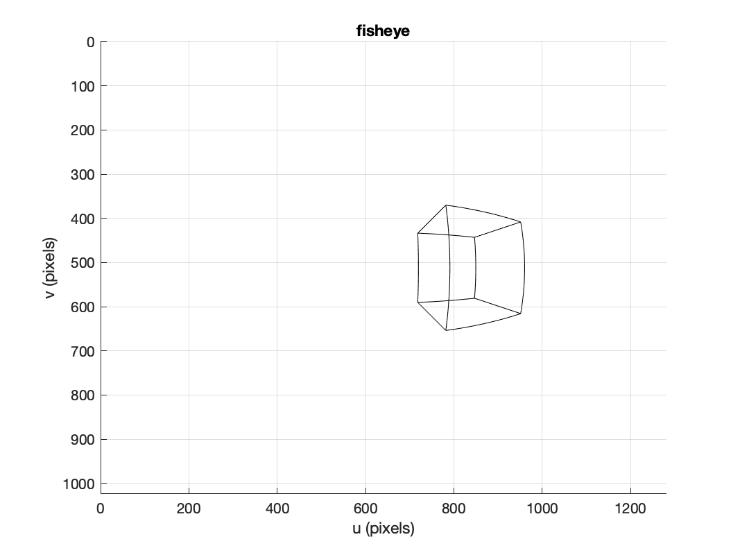
or with a fisheye camera

>> cam = FishEyeCamera('name', 'fisheye', ...

'projection', 'equiangular', ...

'pixel', 10e-6, ...

'resolution', [1280 1024]);

>> [X,Y,Z] = mkcube(0.2, 'centre', [0.2, 0, 0.3], 'edge');

>> cam.mesh(X, Y, Z);

Bundle adjustment

Color space

Plot the CIE chromaticity space

showcolorspace('xy')

lambda = [460:10:540 560:20:600];

[x,y]=lambda2xy(lambda*1e-9);

hold on

plot_point([x y]', 'printf', {' %d', lambda}, 'ko', 'MarkerFaceColor', 'k', 'MarkerSize', 6)

Load the spectrum of sunlight at the Earth's surface and compute the CIE xy chromaticity coordinates

lambda = [400:5:700] * 1e-9; % visible light

sun_at_ground = loadspectrum(lambda, 'solar');

>> lambda2xy(lambda, sun_at_ground)

ans =

0.3327 0.3454

>> colorname(ans, 'xy')

loading rgb.txt

ans =

'antiquewhite4'

Hough transform

im = iread('church.png', 'grey', 'double');

edges = icanny(im);

h = Hough(edges, 'suppress', 10);

lines = h.lines();

idisp(im, 'dark');

lines(1:10).plot('g');

lines = lines.seglength(edges);

lines(1)

k = find( lines.length > 80);

lines(k).plot('b--')

SURF features

We load two images and compute a set of SURF features for each

>> im1 = iread('eiffel2-1.jpg', 'mono', 'double');

>> im2 = iread('eiffel2-2.jpg', 'mono', 'double');

>> sf1 = isurf(im1);

>> sf2 = isurf(im2);

We can match features between images based purely on the similarity of the features, and display the correspondences found

>> m = sf1.match(sf2)

m =

644 corresponding points (listing suppressed)

>> m(1:5)

ans =

(819.56, 358.557) (708.008, 563.342), dist=0.002137

(1028.3, 231.748) (880.14, 461.094), dist=0.004057

(1027.6, 571.118) (885.147, 742.088), dist=0.004297

(927.724, 509.93) (800.833, 692.564), dist=0.004371

(854.35, 401.633) (737.504, 602.187), dist=0.004417

>> idisp({im1, im2})

>> m.subset(100).plot('w')

Clearly there are some bad matches here, but we we can use RANSAC and the epipolar constraint implied by the fundamental matrix to estimate the fundamental matrix and classify correspondences as inliers or outliers

>> F = m.ransac(@fmatrix, 1e-4, 'verbose')

617 trials

295 outliers

0.000145171 final residual

F =

0.0000 -0.0000 0.0087

0.0000 0.0000 -0.0135

-0.0106 0.0116 3.3601

>> m.inlier.subset(100).plot('g')

>> hold on

>> m.outlier.subset(100).plot('r')

>> hold off

where green lines show correct correspondences (inliers) and red lines show bad correspondences (outliers)

Fundamental matrix

What's new

Travis CI is now running on the code base

All code related to pose representation has been split out into the Spatial Math Toolbox. This repo is now a dependency.

Installation

Install from shared MATLAB Drive folder

This will work for MATLAB Online or MATLAB Desktop provided you have MATLAB drive setup.

Click on the appropriate link below and an invitation to share will be emailed to the address associated with your MATLAB account:

Accept the invitation.

A folder named RVC1 or RVC2 will appear in your MATLAB drive folder.

Use the MATLAB file browser and navigate to the folder RVCx/rvctools and double-click the script named startup_rvc.m

Note that this is a combo-installation that includes the Robotics Toolbox (RTB) as well.

Install from github

You need to have a recent version of MATLAB, R2016b or later.

The Machine Vision Toolbox for MATLAB has dependency on two other GitHub repositories: spatial-math and toolbox-common-matlab.

To install the Toolbox on your computer from github follow these simple instructions.

From the shell:

mkdirrvctools

cdrvctools

git clone https://github.com/petercorke/machinevision-toolbox-matlab.git vision

git clone https://github.com/petercorke/spatial-math.git smtb

git clone https://github.com/petercorke/toolbox-common-matlab.git common

make -C vision

The last command builds the MEX files. Then, from within MATLAB

>> addpath rvctools/common % rvctools is the same folder as above

>> startup_rvc

The second line sets up the MATLAB path appropriately but it's only for the current session. You can either:

Repeat this everytime you start MATLAB

Add the MATLAB commands above to your startup.m file

Once you have run startup_rvc, run pathtool and push the Save button, this will save the path settings for subsequent sessions.

Downloading the example images

The Robotics, Vision & Control book (2nd edition) uses a number of example images and image sequences. These are bulky and not really appropriate to keep on Github but you can download them.

There are two zip archives: