


目录
一、Scikit Learn中有关logistics回归函数的介绍... 2
1. 交叉验证... 2
2. 使用搜索进行正则化的 Logistic Regression参数调优... 3
3. 用LogisticRegressionCV实现正则化的 Logistic Regression 参数调优... 6
二、应用举例... 10
1. 读取数据... 10
2. 看各类样本分布是否均衡... 10
3. 特征编码... 10
4. 数据预处理... 10
5. 模型训练... 10
5.1 交叉验证进行 Logistic Regression 参数调优... 10
5.2 使用搜索进行正则化的 Logistic Regression参数调优... 10
5.3 使用LogisticRegressionCV进行正则化的 Logistic Regression 参数调优
... 10
一、Scikit Learn中有关logistics回归函数的介绍
1. 交叉验证
交叉验证用于评估模型性能和进行参数调优(模型选择)。分类任务中交叉验证缺省是采用StratifiedKFold。
sklearn.cross_validation.cross_val_score(estimator, X, y=None, scoring=None, cv=None, n_jobs=1, verbose=0, fit_params=None, pre_dispatch='2*n_jobs')
| Parameters: | estimator : estimator object implementing ‘fit’ The object to use to fit the data. X : array-like The data to fit. Can be, for example a list, or an array at least 2d. y : array-like, optional, default: None The target variable to try to predict in the case of supervised learning. scoring : string, callable or None, optional, default: None A string (see model evaluation documentation) or a scorer callable object / function with signature scorer(estimator, X, y). cv : int, cross-validation generator or an iterable, optional Determines the cross-validation splitting strategy. Possible inputs for cv are:
For integer/None inputs, if the estimator is a classifier and y is either binary or multiclass, StratifiedKFold is used. In all other cases, KFold is used. Refer User Guide for the various cross-validation strategies that can be used here. n_jobs : integer, optional The number of CPUs to use to do the computation. -1 means ‘all CPUs’. verbose : integer, optional The verbosity level. fit_params : dict, optional Parameters to pass to the fit method of the estimator. pre_dispatch : int, or string, optional Controls the number of jobs that get dispatched during parallel execution. Reducing this number can be useful to avoid an explosion of memory consumption when more jobs get dispatched than CPUs can process. This parameter can be: · None, in which case all the jobs are immediately created and spawned. Use this for lightweight and fast-running jobs, to avoid delays due to on-demand spawning of the jobs · An int, giving the exact number of total jobs that are spawned · A string, giving an expression as a function of n_jobs, as in ‘2*n_jobs’ |
| Returns: | scores : array of float, shape=(len(list(cv)),) Array of scores of the estimator for each run of the cross validation. |
2. 使用搜索进行正则化的 Logistic Regression参数调优
sklearn.grid_search.GridSearchCV(estimator, param_grid, scoring=None, fit_params=None, n_jobs=1, iid=True, refit=True, cv=None, verbose=0, pre_dispatch='2*n_jobs', error_score='raise')
| Parameters: | estimator : estimator object. A object of that type is instantiated for each grid point. This is assumed to implement the scikit-learn estimator interface. Either estimator needs to provide a score function, or scoring must be passed. param_grid : dict or list of dictionaries Dictionary with parameters names (string) as keys and lists of parameter settings to try as values, or a list of such dictionaries, in which case the grids spanned by each dictionary in the list are explored. This enables searching over any sequence of parameter settings. scoring : string, callable or None, default=None A string (see model evaluation documentation) or a scorer callable object / function with signature scorer(estimator, X, y). If None, the score method of the estimator is used. fit_params : dict, optional Parameters to pass to the fit method. n_jobs : int, default=1 Number of jobs to run in parallel. Changed in version 0.17: Upgraded to joblib 0.9.3. pre_dispatch : int, or string, optional Controls the number of jobs that get dispatched during parallel execution. Reducing this number can be useful to avoid an explosion of memory consumption when more jobs get dispatched than CPUs can process. This parameter can be: · None, in which case all the jobs are immediately created and spawned. Use this for lightweight and fast-running jobs, to avoid delays due to on-demand spawning of the jobs · An int, giving the exact number of total jobs that are spawned · A string, giving an expression as a function of n_jobs, as in ‘2*n_jobs’ iid : boolean, default=True If True, the data is assumed to be identically distributed across the folds, and the loss minimized is the total loss per sample, and not the mean loss across the folds. cv : int, cross-validation generator or an iterable, optional Determines the cross-validation splitting strategy. Possible inputs for cv are:
For integer/None inputs, if the estimator is a classifier and y is either binary or multiclass, sklearn.model_selection.StratifiedKFold is used. In all other cases, sklearn.model_selection.KFold is used. Refer User Guide for the various cross-validation strategies that can be used here. refit : boolean, default=True Refit the best estimator with the entire dataset. If “False”, it is impossible to make predictions using this GridSearchCV instance after fitting. verbose : integer Controls the verbosity: the higher, the more messages. error_score : ‘raise’ (default) or numeric Value to assign to the score if an error occurs in estimator fitting. If set to ‘raise’, the error is raised. If a numeric value is given, FitFailedWarning is raised. This parameter does not affect the refit step, which will always raise the error. |
| Attributes: | grid_scores_ : list of named tuples Contains scores for all parameter combinations in param_grid. Each entry corresponds to one parameter setting. Each named tuple has the attributes: · parameters, a dict of parameter settings · mean_validation_score, the mean score over the cross-validation folds · cv_validation_scores, the list of scores for each fold best_estimator_ : estimator Estimator that was chosen by the search, i.e. estimator which gave highest score (or smallest loss if specified) on the left out data. Not available if refit=False. best_score_ : float Score of best_estimator on the left out data. best_params_ : dict Parameter setting that gave the best results on the hold out data. scorer_ : function Scorer function used on the held out data to choose the best parameters for the model. |
训练:
fit(X, y=None)
Run fit with all sets of parameters.
| Parameters: | X : array-like, shape = [n_samples, n_features] Training vector, where n_samples is the number of samples and n_features is the number of features. y : array-like, shape = [n_samples] or [n_samples, n_output], optional Target relative to X for classification or regression; None for unsupervised learning. |
3. 用LogisticRegressionCV实现正则化的 Logistic Regression 参数调优
sklearn.linear_model.LogisticRegressionCV(Cs=10, fit_intercept=True, cv=None, dual=False, penalty='l2', scoring=None, solver='lbfgs', tol=0.0001, max_iter=100, class_weight=None, n_jobs=1, verbose=0, refit=True, intercept_scaling=1.0, multi_class='ovr', random_state=None)
| Parameters: | Cs : list of floats | int Each of the values in Cs describes the inverse of regularization strength. If Cs is as an int, then a grid of Cs values are chosen in a logarithmic scale between 1e-4 and 1e4. Like in support vector machines, smaller values specify stronger regularization. fit_intercept : bool, default: True Specifies if a constant (a.k.a. bias or intercept) should be added to the decision function. class_weight : dict or ‘balanced’, optional Weights associated with classes in the form {class_label: weight}. If not given, all classes are supposed to have weight one. The “balanced” mode uses the values of y to automatically adjust weights inversely proportional to class frequencies in the input data as n_samples / (n_classes * np.bincount(y)). Note that these weights will be multiplied with sample_weight (passed through the fit method) if sample_weight is specified. New in version 0.17: class_weight == ‘balanced’ cv : integer or cross-validation generator The default cross-validation generator used is Stratified K-Folds. If an integer is provided, then it is the number of folds used. See the module sklearn.model_selection module for the list of possible cross-validation objects. penalty : str, ‘l1’ or ‘l2’ Used to specify the norm used in the penalization. The ‘newton-cg’, ‘sag’ and ‘lbfgs’ solvers support only l2 penalties. dual : bool Dual or primal formulation. Dual formulation is only implemented for l2 penalty with liblinear solver. Prefer dual=False when n_samples > n_features. scoring : callabale Scoring function to use as cross-validation criteria. For a list of scoring functions that can be used, look at sklearn.metrics. The default scoring option used is accuracy_score. solver : {‘newton-cg’, ‘lbfgs’, ‘liblinear’, ‘sag’} Algorithm to use in the optimization problem.
faster for large ones.
multinomial loss; ‘liblinear’ is limited to one-versus-rest schemes.
not handle warm-starting. Note that ‘sag’ fast convergence is only guaranteed on features with approximately the same scale. You can preprocess the data with a scaler from sklearn.preprocessing. New in version 0.17: Stochastic Average Gradient descent solver. tol : float, optional Tolerance for stopping criteria. max_iter : int, optional Maximum number of iterations of the optimization algorithm. n_jobs : int, optional Number of CPU cores used during the cross-validation loop. If given a value of -1, all cores are used. verbose : int For the ‘liblinear’, ‘sag’ and ‘lbfgs’ solvers set verbose to any positive number for verbosity. refit : bool If set to True, the scores are averaged across all folds, and the coefs and the C that corresponds to the best score is taken, and a final refit is done using these parameters. Otherwise the coefs, intercepts and C that correspond to the best scores across folds are averaged. multi_class : str, {‘ovr’, ‘multinomial’} Multiclass option can be either ‘ovr’ or ‘multinomial’. If the option chosen is ‘ovr’, then a binary problem is fit for each label. Else the loss minimised is the multinomial loss fit across the entire probability distribution. Works only for the ‘newton-cg’, ‘sag’ and ‘lbfgs’ solver. New in version 0.18: Stochastic Average Gradient descent solver for ‘multinomial’ case. intercept_scaling : float, default 1. Useful only when the solver ‘liblinear’ is used and self.fit_intercept is set to True. In this case, x becomes [x, self.intercept_scaling], i.e. a “synthetic” feature with constant value equal to intercept_scaling is appended to the instance vector. The intercept becomes intercept_scaling * synthetic_feature_weight. Note! the synthetic feature weight is subject to l1/l2 regularization as all other features. To lessen the effect of regularization on synthetic feature weight (and therefore on the intercept) intercept_scaling has to be increased. random_state : int seed, RandomState instance, or None (default) The seed of the pseudo random number generator to use when shuffling the data. |
| Attributes: | coef_ : array, shape (1, n_features) or (n_classes, n_features) Coefficient of the features in the decision function. coef_ is of shape (1, n_features) when the given problem is binary. coef_ is readonly property derived from raw_coef_ that follows the internal memory layout of liblinear. intercept_ : array, shape (1,) or (n_classes,) Intercept (a.k.a. bias) added to the decision function. It is available only when parameter intercept is set to True and is of shape(1,) when the problem is binary. Cs_ : array Array of C i.e. inverse of regularization parameter values used for cross-validation. coefs_paths_ : array, shape (n_folds, len(Cs_), n_features) or (n_folds, len(Cs_), n_features + 1) dict with classes as the keys, and the path of coefficients obtained during cross-validating across each fold and then across each Cs after doing an OvR for the corresponding class as values. If the ‘multi_class’ option is set to ‘multinomial’, then the coefs_paths are the coefficients corresponding to each class. Each dict value has shape (n_folds, len(Cs_), n_features) or (n_folds, len(Cs_), n_features + 1) depending on whether the intercept is fit or not. scores_ : dict dict with classes as the keys, and the values as the grid of scores obtained during cross-validating each fold, after doing an OvR for the corresponding class. If the ‘multi_class’ option given is ‘multinomial’ then the same scores are repeated across all classes, since this is the multinomial class. Each dict value has shape (n_folds, len(Cs)) C_ : array, shape (n_classes,) or (n_classes - 1,) Array of C that maps to the best scores across every class. If refit is set to False, then for each class, the best C is the average of the C’s that correspond to the best scores for each fold. n_iter_ : array, shape (n_classes, n_folds, n_cs) or (1, n_folds, n_cs) Actual number of iterations for all classes, folds and Cs. In the binary or multinomial cases, the first dimension is equal to 1. |
二、应用举例
Kaggle 2015年举办的Otto Group Product Classification Challenge竞赛数据为例。
1. 读取数据
# 首先 import 必要的模块 import pandas as pd import numpy as np from sklearn.model_selection import GridSearchCV #评价指标为logloss from sklearn.metrics import log_loss from matplotlib import pyplot import seaborn as sns %matplotlib inline
# 读取数据
dpath = './data/'
train = pd.read_csv(dpath +"Otto_train.csv")
train.head()
2. 看各类样本分布是否均衡
# Target 分布,看看各类样本分布是否均衡
sns.countplot(train.target);
pyplot.xlabel('target');
pyplot.ylabel('Number of occurrences');
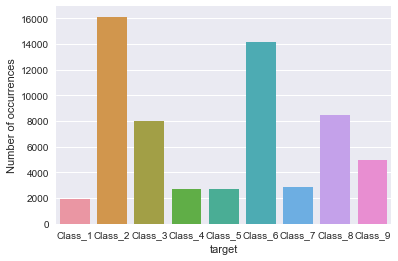
各类样本不均衡。交叉验证对分类任务缺省的是采用StratifiedKFold,在每折采样时根据各类样本按比例采样
3. 特征编码
# 将类别字符串变成数字
y_train = train['target']
y_train = y_train.map(lambda s: s[6:])      # 对于s使用s[6:]来代替
y_train = y_train.map(lambda s: int(s)-1)   # 对于s使用int(s)-1来代替

train = train.drop(["id", "target"], axis=1) # 去掉 "id", "target"这2列
X_train = np.array(train)[0:2000,:] # 转为数组
4. 数据预处理
# 数据标准化
from sklearn.preprocessing import StandardScaler

# 初始化特征的标准化器
ss_X = StandardScaler()

# 分别对训练数据的特征进行标准化处理
X_train = ss_X.fit_transform(X_train)
5. 模型训练
5.1 交叉验证进行 Logistic Regression 参数调优
from sklearn.linear_model import LogisticRegression
lr= LogisticRegression()
# 交叉验证用于评估模型性能和进行参数调优(模型选择)
#分类任务中交叉验证缺省是采用StratifiedKFold
from sklearn.cross_validation import cross_val_score
# cross_val_score(estimator, X, y=None, scoring=None, cv=None, ...)
# estimator: 模型,X:特征,y:标签,scoring:分数规则,cv:k折交叉验证
scores = cross_val_score(lr, X_train, y_train, cv=5, scoring='accuracy')
print 'accuracy of each fold is: '
print(scores)
print'cv accuracy is:', scores.mean()
accuracy of each fold is:
[ 0.97755611  0.9925      0.9775      0.9875      0.98746867]
cv accuracy is: 0.984504956281
5.2 使用搜索进行正则化的 Logistic Regression参数调优
from sklearn.model_selection import GridSearchCV
from sklearn.linear_model import LogisticRegression

#需要调优的参数
# 请尝试将L1正则和L2正则分开,并配合合适的优化求解算法(slover)
#tuned_parameters = {'penalty':['l1','l2'],
#                   'C': [0.001, 0.01, 0.1, 1, 10, 100, 1000]
#                   }
penaltys = ['l1','l2']
Cs = [0.001, 0.01, 0.1, 1, 10, 100, 1000]
tuned_parameters = dict(penalty = penaltys, C = Cs)

lr_penalty= LogisticRegression()
# GridSearchCV(estimator, param_grid, ... cv=None, ...)
# estimator: 模型, param_grid:字典类型的参数, cv:k折交叉验证
grid= GridSearchCV(lr_penalty, tuned_parameters, cv=5)
grid.fit(X_train,y_train) # 网格搜索训练
grid.cv_results_ #训练的结果
{'mean_fit_time': array([ 0.00779996,  0.01719995,  0.01200004,  0.02780004,  0.01939998,
         0.03739996,  0.048     ,  0.05899997,  0.21480007,  0.12020001,
         0.4348001 ,  0.13859997,  0.39040003,  0.15320001]),
 'mean_score_time': array([ 0.00039997,  0.00040002,  0.00059996,  0.00059996,  0.00059996,
         0.0006    ,  0.00039997,  0.00019999,  0.00040002,  0.00040002,
         0.0006    ,  0.0006    ,  0.00079994,  0.00099993]),
 'mean_test_score': array([ 0.9645,  0.976 ,  0.9645,  0.9805,  0.9785,  0.9805,  0.985 ,
         0.9845,  0.983 ,  0.9805,  0.98  ,  0.977 ,  0.9775,  0.974 ]),
 'mean_train_score': array([ 0.96450007,  0.98012508,  0.96512492,  0.98399976,  0.98137492,
         0.987875  ,  0.99462492,  0.9945    ,  0.999625  ,  0.99824992,
         1.        ,  1.        ,  1.        ,  1.        ]),
 'param_C': masked_array(data = [0.001 0.001 0.01 0.01 0.1 0.1 1 1 10 10 100 100 1000 1000],
              mask = [False False False False False False False False False False False False
  False False],
        fill_value = ?),
 'param_penalty': masked_array(data = ['l1' 'l2' 'l1' 'l2' 'l1' 'l2' 'l1' 'l2' 'l1' 'l2' 'l1' 'l2' 'l1' 'l2'],
              mask = [False False False False False False False False False False False False
  False False],
        fill_value = ?),
 'params': ({'C': 0.001, 'penalty': 'l1'},
  {'C': 0.001, 'penalty': 'l2'},
  {'C': 0.01, 'penalty': 'l1'},
  {'C': 0.01, 'penalty': 'l2'},
  {'C': 0.1, 'penalty': 'l1'},
  {'C': 0.1, 'penalty': 'l2'},
  {'C': 1, 'penalty': 'l1'},
  {'C': 1, 'penalty': 'l2'},
  {'C': 10, 'penalty': 'l1'},
  {'C': 10, 'penalty': 'l2'},
  {'C': 100, 'penalty': 'l1'},
  {'C': 100, 'penalty': 'l2'},
  {'C': 1000, 'penalty': 'l1'},
  {'C': 1000, 'penalty': 'l2'}),
 'rank_test_score': array([13, 11, 13,  4,  8,  4,  1,  2,  3,  4,  7, 10,  9, 12]),
 'split0_test_score': array([ 0.96259352,  0.96758105,  0.96259352,  0.97506234,  0.97256858,
         0.97506234,  0.97755611,  0.97755611,  0.97755611,  0.98004988,
         0.97007481,  0.97256858,  0.97506234,  0.97506234]),
 'split0_train_score': array([ 0.96497811,  0.98186366,  0.9656035 ,  0.98373984,  0.98186366,
         0.98811757,  0.99437148,  0.99437148,  0.99937461,  0.99749844,
         1.        ,  1.        ,  1.        ,  1.        ]),
 'split1_test_score': array([ 0.965 ,  0.9825,  0.965 ,  0.9875,  0.9825,  0.9875,  0.99  ,
         0.9925,  0.9825,  0.9825,  0.9775,  0.9825,  0.9725,  0.9775]),
 'split1_train_score': array([ 0.964375,  0.97625 ,  0.965   ,  0.983125,  0.979375,  0.986875,
         0.994375,  0.994375,  0.999375,  0.996875,  1.      ,  1.      ,
         1.      ,  1.      ]),
 'split2_test_score': array([ 0.965 ,  0.9825,  0.965 ,  0.9825,  0.9825,  0.9825,  0.9825,
         0.9775,  0.9775,  0.97  ,  0.9775,  0.9675,  0.975 ,  0.965 ]),
 'split2_train_score': array([ 0.964375,  0.980625,  0.964375,  0.98375 ,  0.981875,  0.98875 ,
         0.99625 ,  0.995625,  1.      ,  0.999375,  1.      ,  1.      ,
         1.      ,  1.      ]),
 'split3_test_score': array([ 0.965 ,  0.9775,  0.965 ,  0.9825,  0.985 ,  0.9825,  0.99  ,
         0.9875,  0.9875,  0.985 ,  0.985 ,  0.98  ,  0.985 ,  0.975 ]),
 'split3_train_score': array([ 0.964375,  0.980625,  0.964375,  0.98375 ,  0.98125 ,  0.9875  ,
         0.993125,  0.99375 ,  1.      ,  0.999375,  1.      ,  1.      ,
         1.      ,  1.      ]),
 'split4_test_score': array([ 0.96491228,  0.96992481,  0.96491228,  0.97493734,  0.96992481,
         0.97493734,  0.98496241,  0.98746867,  0.98997494,  0.98496241,
         0.98997494,  0.98245614,  0.97994987,  0.97744361]),
 'split4_train_score': array([ 0.96439725,  0.98126171,  0.96627108,  0.98563398,  0.98251093,
         0.98813242,  0.99500312,  0.99437851,  0.99937539,  0.99812617,
         1.        ,  1.        ,  1.        ,  1.        ]),
 'std_fit_time': array([ 0.0011662 ,  0.00116623,  0.00063249,  0.00305936,  0.00185475,
         0.00205906,  0.00460443,  0.0018974 ,  0.04810566,  0.01215555,
         0.17968574,  0.01993598,  0.10196788,  0.02121689]),
 'std_score_time': array([ 0.00048986,  0.00048992,  0.00048986,  0.00048986,  0.00048986,
         0.0004899 ,  0.00048986,  0.00039997,  0.00048992,  0.00048992,
         0.0004899 ,  0.0004899 ,  0.00039997,  0.        ]),
 'std_test_score': array([ 0.00095533,  0.00623894,  0.00095533,  0.00484784,  0.00604764,
         0.00484784,  0.00472867,  0.00598547,  0.00507914,  0.00555997,
         0.00686303,  0.00598133,  0.00445968,  0.00463055]),
 'std_train_score': array([ 0.00023917,  0.00199152,  0.00073254,  0.00085184,  0.00107655,
         0.00063739,  0.00101591,  0.00061238,  0.00030619,  0.00100021,
         0.        ,  0.        ,  0.        ,  0.        ])}
# examine the best model
print(grid.best_score_)  # 最好的分数
print(grid.best_params_) # 最好的参数
0.754775526035
{'penalty': 'l1', 'C': 100}
如果最佳值在候选参数的边缘,最好再尝试更大的候选参数或更小的候选参数,直到找到拐点。
5.3 使用LogisticRegressionCV进行正则化的 Logistic Regression 参数调优
from sklearn.linear_model import LogisticRegressionCV

Cs = [1, 10,100,1000]

# 大量样本(7W)、高维度(93),L1正则 --> 可选用saga优化求解器(0.19版本新功能)
lr_cv = LogisticRegressionCV(Cs=Cs, cv = 5, penalty='l1', solver='liblinear', multi_class='ovr')
lr_cv.fit(X_train, y_train)
LogisticRegressionCV(Cs=[1, 10, 100, 1000], class_weight=None, cv=5,
           dual=False, fit_intercept=True, intercept_scaling=1.0,
           max_iter=100, multi_class='ovr', n_jobs=1, penalty='l1',
           random_state=None, refit=True, scoring=None, solver='liblinear',
           tol=0.0001, verbose=0)
lr_cv.scores_ # 网格中每次迭代的分数
{1: array([[ 0.97755611,  0.97755611,  0.97007481,  0.97506234],
        [ 0.99      ,  0.9825    ,  0.9775    ,  0.975     ],
        [ 0.9825    ,  0.9775    ,  0.9775    ,  0.975     ],
        [ 0.99      ,  0.9875    ,  0.985     ,  0.985     ],
        [ 0.98496241,  0.98997494,  0.98997494,  0.97994987]])}


 1143
1143


 被折叠的 条评论
为什么被折叠?
被折叠的 条评论
为什么被折叠?
 到【灌水乐园】发言


