Keras实现DeepLabV3+多类语义分割

基于Keras框架，实现用于多类语义分割的DeepLabV3+模型，DeepLabV3+是一个在语义分割基准测试中表现优异的全卷积网络。

本文将使用Crowd Instance-level Human Parsing（CIHP）数据集来训练模型。CIHP数据集有38,280张不同的人类图像，并对每张图像都标注了20个类别的像素级标签和实例级标签。CIHP数据集可以用于“人体部位分割（human part segmentation）”任务。 

CIHP数据集

登录后复制

import os  
import cv2  
import numpy as np  
from glob import glob  
from scipy.io import loadmat  
import matplotlib.pyplot as plt  
  
import tensorflow as tf  
from tensorflow import keras  
from tensorflow.keras import layers

• 1.
• 2.
• 3.
• 4.
• 5.
• 6.
• 7.
• 8.
• 9.
• 10.

CIHP数据集下载地址为：https://www.cvmart.net/dataSets/detail/608

登录后复制

!gdown https://drive.google.com/uc?id=1B9A9UCJYMwTL4oBEo4RZfbMZMaZhKJaz  
!unzip -q instance-level-human-parsing.zip

• 1.
• 2.

创建TensorFlow数据集

在包含38,280张图像的整个CIHP数据集上进行训练需要大量时间，因此在本例中，仅使用200张图像的较小子集来训练模型。

登录后复制

IMAGE_SIZE = 512  
BATCH_SIZE = 4  
NUM_CLASSES = 20  
DATA_DIR = "./instance-level_human_parsing/instance-level_human_parsing/Training"  
NUM_TRAIN_IMAGES = 1000  
NUM_VAL_IMAGES = 50  
  
train_images = sorted(glob(os.path.join(DATA_DIR, "Images/*")))[:NUM_TRAIN_IMAGES]  
train_masks = sorted(glob(os.path.join(DATA_DIR, "Category_ids/*")))[:NUM_TRAIN_IMAGES]  
val_images = sorted(glob(os.path.join(DATA_DIR, "Images/*")))[  
    NUM_TRAIN_IMAGES : NUM_VAL_IMAGES + NUM_TRAIN_IMAGES  
]  
val_masks = sorted(glob(os.path.join(DATA_DIR, "Category_ids/*")))[  
    NUM_TRAIN_IMAGES : NUM_VAL_IMAGES + NUM_TRAIN_IMAGES  
]  
  
  
def read_image(image_path, mask=False):  
    image = tf.io.read_file(image_path)  
    if mask:  
        image = tf.image.decode_png(image, channels=1)  
        image.set_shape([None, None, 1])  
        image = tf.image.resize(images=image, size=[IMAGE_SIZE, IMAGE_SIZE])  
    else:  
        image = tf.image.decode_png(image, channels=3)  
        image.set_shape([None, None, 3])  
        image = tf.image.resize(images=image, size=[IMAGE_SIZE, IMAGE_SIZE])  
        image = tf.keras.applications.resnet50.preprocess_input(image)  
    return image  
  
  
def load_data(image_list, mask_list):  
    image = read_image(image_list)  
    mask = read_image(mask_list, mask=True)  
    return image, mask  
  
  
def data_generator(image_list, mask_list):  
    dataset = tf.data.Dataset.from_tensor_slices((image_list, mask_list))  
    dataset = dataset.map(load_data, num_parallel_calls=tf.data.AUTOTUNE)  
    dataset = dataset.batch(BATCH_SIZE, drop_remainder=True)  
    return dataset  
  
  
train_dataset = data_generator(train_images, train_masks)  
val_dataset = data_generator(val_images, val_masks)  
  
print("Train Dataset:", train_dataset)  
print("Val Dataset:", val_dataset)

• 1.
• 2.
• 3.
• 4.
• 5.
• 6.
• 7.
• 8.
• 9.
• 10.
• 11.
• 12.
• 13.
• 14.
• 15.
• 16.
• 17.
• 18.
• 19.
• 20.
• 21.
• 22.
• 23.
• 24.
• 25.
• 26.
• 27.
• 28.
• 29.
• 30.
• 31.
• 32.
• 33.
• 34.
• 35.
• 36.
• 37.
• 38.
• 39.
• 40.
• 41.
• 42.
• 43.
• 44.
• 45.
• 46.
• 47.
• 48.
• 49.

构建DeepLabV3+模型

DeepLabv3+通过添加编码器-解码器结构（encoder-decoder structure ）扩展了DeepLabv3。编码器模块通过在多个尺度上应用扩张卷积来处理多尺度上下文信息，而解码器模块则沿着对象边界细化分割结果。

模型结构

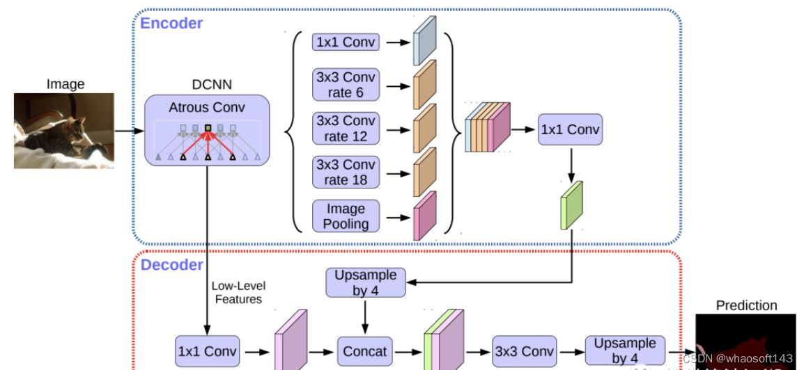
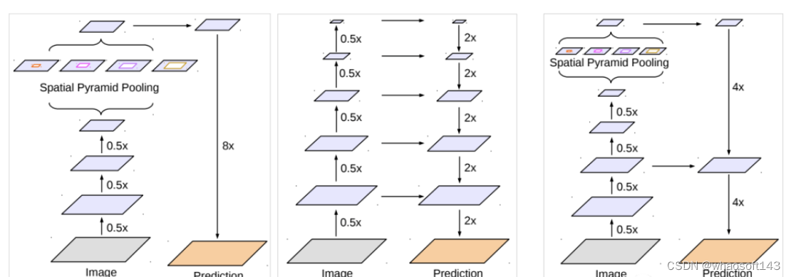
DeepLabv3+ 模型的整体架构如上图所示，它的 Encoder 的主体是带有空洞卷积的 DCNN，可以采用常用的分类网络如 ResNet，然后是带有空洞卷积的空间金字塔池化模块（Atrous Spatial Pyramid Pooling，ASPP），主要是为了引入多尺度信息；相比DeepLabv3，v3+ 引入了 Decoder 模块，其将底层特征与高层特征进一步融合，提升分割边界准确度。从某种意义上看，DeepLabv3+ 在 DilatedFCN 基础上引入了 EcoderDecoder 的思路。对于 DilatedFCN，主要是修改分类网络的后面 block，用空洞卷积来替换 stride=2 的下采样层，如下图所示：其中 (a) 是原始 FCN，由于下采样的存在，特征图不断降低；而 (b) 为 DilatedFCN，在第 block3 后引入空洞卷积，在维持特征图大小的同时保证了感受野和原始网络一致。 

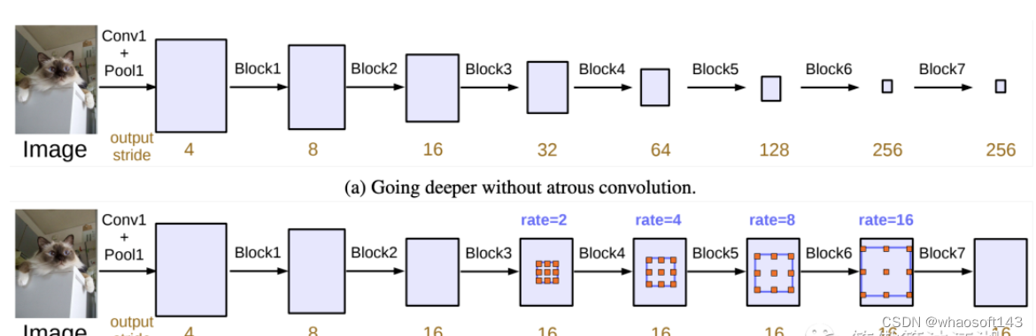
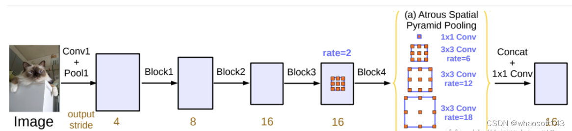
在 DeepLab 中，将输入图片与输出特征图的尺度之比记为 output_stride，如上图的 output_stride 为16，如果加上 ASPP 结构，就变成如下图所示。其实这就是 DeepLabv3 结构，v3+ 只不过是增加了 Decoder 模块。这里的 DCNN 可以是任意的分类网络，一般又称为 backbone，如采用 ResNet 网络。

扩张卷积

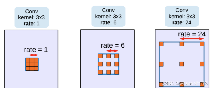
随着网络的深入，使用扩张卷积（Dilated Convolution），也可以称为空洞卷积（Atrous Convolution），可以保持步幅不变，但视野更大，而不增加参数数量或计算量。此外，它支持更大的输出特征映射，这对语义分割很有用。空洞卷积是 DeepLab 模型的关键之一，它可以在不改变特征图大小的同时控制感受野，这有利于提取多尺度信息。空洞卷积如下图所示，其中rate（r）控制着感受野的大小，r 越大感受野越大。通常的 CNN 分类网络的 output_stride=32，若希望 DilatedFCN 的 output_stride=16，只需要将最后一个下采样层的 stride 设置为1，并且后面所有卷积层的 r 设置为 2，这样保证感受野没有发生变化。对于 output_stride=8，需要将最后的两个下采样层的 stride 改为 1，并且后面对应的卷积层的 rate 分别设为 2 和 4。另外一点，DeepLabv3 中提到了采用 multi-grid 方法，针对 ResNet 网络，最后的 3 个级联 block 采用不同 rate，若 output_stride=16 且 multi_grid = (1, 2, 4), 那么最后的 3 个 block 的 rate= 2 · (1, 2, 4) = (2, 4, 8)。这比直接采用 (1, 1, 1) 要更有效一些，不过结果相差不是太大。

扩展空间金字塔池化

使用扩展空间金字塔池化（Dilated Spatial Pyramid Pooling）的原因是，随着采样率的增大，有效过滤器权重的数量(即，应用于有效特征区域的权重，而不是填充的零)变得越来越小。SPP-Net是2015年发表在IEEE上的论文。在此之前，所有的神经网络都是需要输入固定尺寸的图片，比如 224×224（ImageNet）、32×32 (LenNet)、96×96 等。这样对于我们希望检测各种大小的图片的时候，需要经过 crop，或者 warp 等一系列操作，这都在一定程度上导致图片信息的丢失和变形，限制了识别精确度。而且，从生理学角度出发，人眼看到一个图片时，大脑会首先认为这是一个整体，而不会进行 crop 和 warp，所以更有可能的是，我们的大脑通过搜集一些浅层的信息，在更深层才识别出这些任意形状的目标。ASPP(Atrous Spatial Pyramid Pooling)是 DeepLab 中用于语义分割的一个模块。由于被检测物体具有不同的尺度，给分割增加了难度。一种方法是通过 rescale 图片，分别经过 DCNN(Deep Convolutional Neural Network) 检测，然后融合，但这种方法计算量大。DeepLab 就设计了一个 ASPP 的模块，既能得到多尺度信息，计算量又比较小，其中还使用了空洞卷积(Atrous Convolution)的方法在 DeepLab 中，采用空间金字塔池化模块来进一步提取多尺度信息，这里是采用不同 rate 的空洞卷积来实现这一点。ASPP 模块主要包含以下几个部分：

1. 一个 1×1 卷积层，以及三个 3x3 的空洞卷积，对于 output_stride=16，其 rate 为(6, 12, 18) ，若 output_stride=8，rate 加倍（这些卷积层的输出 channel 数均为 256，并且含有 BN 层）；
2. 一个全局平均池化层得到 image-level 特征，然后送入 1x1 卷积层（输出 256 个 channel），并双线性插值到原始大小；
3. 将前两步得到的 4 个不同尺度的特征在 channel 维度 concat 在一起，然后送入 1x1 的卷积进行融合并得到 256-channel 的新特征。

DeepLabv3+改进了DeepLabv3，采用了空间金字塔池化模块(a)， (b)DeepLabv3+包含编码器模块提供了丰富的语义信息，而解码器模块简单有效地恢复了详细的对象边界，编码器模块可以通过空洞卷积（atrous convolution）在任意分辨率提取特征

Decoder

对于 DeepLabv3，经过 ASPP 模块得到的特征图的 output_stride 为 8 或者 16，其经过 1x1 的分类层后直接双线性插值到原始图片大小，这是一种非常暴力的 decoder 方法，特别是 output_stride=16。然而这并不利于得到较精细的分割结果，故 v3+ 模型中借鉴了 EncoderDecoder 结构，引入了新的 Decoder 模块，如下图所示。首先将 encoder 得到的特征双线性插值得到 4x 的特征，然后与 encoder 中对应大小的低级特征 concat，如 ResNet 中的 Conv2 层，由于 encoder 得到的特征数只有 256，而低级特征维度可能会很高，为了防止 encoder 得到的高级特征被弱化，先采用 1x1 卷积对低级特征进行降维（paper 中输出维度为 48）。两个特征 concat 后，再采用 3x3 卷积进一步融合特征，最后再双线性插值得到与原始图片相同大小的分割预测。

改进的Xception

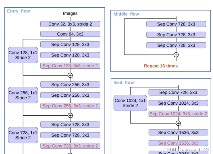
DeepLabv3 所采用的 backbone 是 ResNet 网络，在 v3+ 模型作者尝试了改进的 Xception，Xception 网络主要采用 depthwise separable convolution，这使得 Xception 计算量更小。改进的 Xception 主要体现在以下几点：

1. 参考 MSRA 的修改（Deformable Convolutional Networks），增加了更多的层；
2. 所有的最大池化层使用 stride=2 的 depthwise separable convolutions 替换，这样可以改成空洞卷积 ；
3. 与 MobileNet 类似，在 3x3 depthwise convolution 后增加 BN 和 ReLU。

采用改进的 Xception 网络作为 backbone，DeepLab 网络分割效果上有一定的提升。作者还尝试了在 ASPP 中加入 depthwise separable convolution，发现在基本不影响模型效果的前提下减少计算量。

登录后复制

def convolution_block(  
    block_input,  
    num_filters=256,  
    kernel_size=3,  
    dilation_rate=1,  
    padding="same",  
    use_bias=False,  
):  
    x = layers.Conv2D(  
        num_filters,  
        kernel_size=kernel_size,  
        dilation_rate=dilation_rate,  
        padding="same",  
        use_bias=use_bias,  
        kernel_initializer=keras.initializers.HeNormal(),  
    )(block_input)  
    x = layers.BatchNormalization()(x)  
    return tf.nn.relu(x)  
  
  
def DilatedSpatialPyramidPooling(dspp_input):  
    dims = dspp_input.shape  
    x = layers.AveragePooling2D(pool_size=(dims[-3], dims[-2]))(dspp_input)  
    x = convolution_block(x, kernel_size=1, use_bias=True)  
    out_pool = layers.UpSampling2D(  
        size=(dims[-3] // x.shape[1], dims[-2] // x.shape[2]), interpolation="bilinear",  
    )(x)  
  
    out_1 = convolution_block(dspp_input, kernel_size=1, dilation_rate=1)  
    out_6 = convolution_block(dspp_input, kernel_size=3, dilation_rate=6)  
    out_12 = convolution_block(dspp_input, kernel_size=3, dilation_rate=12)  
    out_18 = convolution_block(dspp_input, kernel_size=3, dilation_rate=18)  
  
    x = layers.Concatenate(axis=-1)([out_pool, out_1, out_6, out_12, out_18])  
    output = convolution_block(x, kernel_size=1)  
    return output

• 1.
• 2.
• 3.
• 4.
• 5.
• 6.
• 7.
• 8.
• 9.
• 10.
• 11.
• 12.
• 13.
• 14.
• 15.
• 16.
• 17.
• 18.
• 19.
• 20.
• 21.
• 22.
• 23.
• 24.
• 25.
• 26.
• 27.
• 28.
• 29.
• 30.
• 31.
• 32.
• 33.
• 34.
• 35.
• 36.

编码器特征首先双线性上采样4倍，然后与网络骨干网中具有相同空间分辨率的相应低级特征连接。对于这个例子，我们使用在ImageNet上预训练的ResNet50作为骨干模型，我们使用来自骨干的conv4_block6_2_relu块的低级特征。

登录后复制

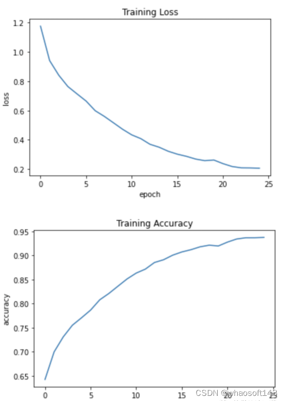
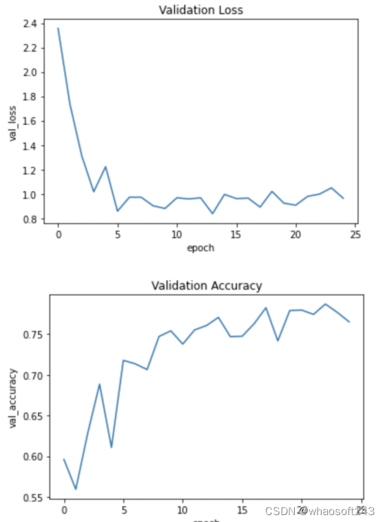
def DeeplabV3Plus(image_size, num_classes):  
    model_input = keras.Input(shape=(image_size, image_size, 3))  
    resnet50 = keras.applications.ResNet50(  
        weights="imagenet", include_top=False, input_tensor=model_input  
    )  
    x = resnet50.get_layer("conv4_block6_2_relu").output  
    x = DilatedSpatialPyramidPooling(x)  
  
    input_a = layers.UpSampling2D(  
        size=(image_size // 4 // x.shape[1], image_size // 4 // x.shape[2]),  
        interpolation="bilinear",  
    )(x)  
    input_b = resnet50.get_layer("conv2_block3_2_relu").output  
    input_b = convolution_block(input_b, num_filters=48, kernel_size=1)  
  
    x = layers.Concatenate(axis=-1)([input_a, input_b])  
    x = convolution_block(x)  
    x = convolution_block(x)  
    x = layers.UpSampling2D(  
        size=(image_size // x.shape[1], image_size // x.shape[2]),  
        interpolation="bilinear",  
    )(x)  
    model_output = layers.Conv2D(num_classes, kernel_size=(1, 1), padding="same")(x)  
    return keras.Model(inputs=model_input, outputs=model_output)  
  
  
model = DeeplabV3Plus(image_size=IMAGE_SIZE, num_classes=NUM_CLASSES)  
model.summary()

• 1.
• 2.
• 3.
• 4.
• 5.
• 6.
• 7.
• 8.
• 9.
• 10.
• 11.
• 12.
• 13.
• 14.
• 15.
• 16.
• 17.
• 18.
• 19.
• 20.
• 21.
• 22.
• 23.
• 24.
• 25.
• 26.
• 27.
• 28.

模型训练

我们使用稀疏分类交叉熵作为损失函数，Adam作为优化器来训练模型。

登录后复制

loss = keras.losses.SparseCategoricalCrossentropy(from_logits=True)  
model.compile(  
    optimizer=keras.optimizers.Adam(learning_rate=0.001),  
    loss=loss,  
    metrics=["accuracy"],  
)  
  
history = model.fit(train_dataset, validation_data=val_dataset, epochs=25)  
  
plt.plot(history.history["loss"])  
plt.title("Training Loss")  
plt.ylabel("loss")  
plt.xlabel("epoch")  
plt.show()  
  
plt.plot(history.history["accuracy"])  
plt.title("Training Accuracy")  
plt.ylabel("accuracy")  
plt.xlabel("epoch")  
plt.show()  
  
plt.plot(history.history["val_loss"])  
plt.title("Validation Loss")  
plt.ylabel("val_loss")  
plt.xlabel("epoch")  
plt.show()  
  
plt.plot(history.history["val_accuracy"])  
plt.title("Validation Accuracy")  
plt.ylabel("val_accuracy")  
plt.xlabel("epoch")  
plt.show()

• 1.
• 2.
• 3.
• 4.
• 5.
• 6.
• 7.
• 8.
• 9.
• 10.
• 11.
• 12.
• 13.
• 14.
• 15.
• 16.
• 17.
• 18.
• 19.
• 20.
• 21.
• 22.
• 23.
• 24.
• 25.
• 26.
• 27.
• 28.
• 29.
• 30.
• 31.
• 32.

 

 

推理过程

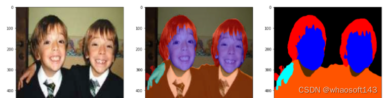
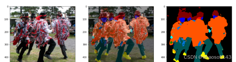
来自模型的原始预测表示一个单热编码的形状张量(N, 512,512,20)，其中20个通道中的每一个都是对应于预测标签的二进制掩码。为了使结果可视化，我们将其绘制为RGB分割掩码，其中每个像素都由对应于预测的特定标签的唯一颜色表示。我们可以从human_colormap.mat中找到每个标签对应的颜色。Mat文件作为数据集的一部分提供。我们还将在输入图像上绘制一个RGB分割掩码的覆盖，因为这进一步帮助我们更直观地识别图像中存在的不同类别。

登录后复制

# Loading the Colormap  
colormap = loadmat(  
    "./instance-level_human_parsing/instance-level_human_parsing/human_colormap.mat"  
)["colormap"]  
colormap = colormap * 100  
colormap = colormap.astype(np.uint8)  
  
  
def infer(model, image_tensor):  
    predictions = model.predict(np.expand_dims((image_tensor), axis=0))  
    predictions = np.squeeze(predictions)  
    predictions = np.argmax(predictions, axis=2)  
    return predictions  
  
  
def decode_segmentation_masks(mask, colormap, n_classes):  
    r = np.zeros_like(mask).astype(np.uint8)  
    g = np.zeros_like(mask).astype(np.uint8)  
    b = np.zeros_like(mask).astype(np.uint8)  
    for l in range(0, n_classes):  
        idx = mask == l  
        r[idx] = colormap[l, 0]  
        g[idx] = colormap[l, 1]  
        b[idx] = colormap[l, 2]  
    rgb = np.stack([r, g, b], axis=2)  
    return rgb  
  
  
def get_overlay(image, colored_mask):  
    image = tf.keras.preprocessing.image.array_to_img(image)  
    image = np.array(image).astype(np.uint8)  
    overlay = cv2.addWeighted(image, 0.35, colored_mask, 0.65, 0)  
    return overlay  
  
  
def plot_samples_matplotlib(display_list, figsize=(5, 3)):  
    _, axes = plt.subplots(nrows=1, ncols=len(display_list), figsize=figsize)  
    for i in range(len(display_list)):  
        if display_list[i].shape[-1] == 3:  
            axes[i].imshow(tf.keras.preprocessing.image.array_to_img(display_list[i]))  
        else:  
            axes[i].imshow(display_list[i])  
    plt.show()  
  
  
def plot_predictions(images_list, colormap, model):  
    for image_file in images_list:  
        image_tensor = read_image(image_file)  
        prediction_mask = infer(image_tensor=image_tensor, model=model)  
        prediction_colormap = decode_segmentation_masks(prediction_mask, colormap, 20)  
        overlay = get_overlay(image_tensor, prediction_colormap)  
        plot_samples_matplotlib(  
            [image_tensor, overlay, prediction_colormap], figsize=(18, 14)  
        )

• 1.
• 2.
• 3.
• 4.
• 5.
• 6.
• 7.
• 8.
• 9.
• 10.
• 11.
• 12.
• 13.
• 14.
• 15.
• 16.
• 17.
• 18.
• 19.
• 20.
• 21.
• 22.
• 23.
• 24.
• 25.
• 26.
• 27.
• 28.
• 29.
• 30.
• 31.
• 32.
• 33.
• 34.
• 35.
• 36.
• 37.
• 38.
• 39.
• 40.
• 41.
• 42.
• 43.
• 44.
• 45.
• 46.
• 47.
• 48.
• 49.
• 50.
• 51.
• 52.
• 53.
• 54.

测试一下

登录后复制

plot_predictions(train_images[:4], colormap, model=model)

• 1.

 

原创作者: whaosoft 转载于: https://blog.51cto.com/whaosoft/11639924