Histogram equalization

      This method usually increases the global contrast of many images, especially when the usable data of the image is represented by close contrast values. Through this adjustment, the intensities can be better distributed on the histogram. This allows for areas of lower local contrast to gain a higher contrast. Histogram equalization accomplishes this by effectively spreading out the most frequent intensity values.

      The method is useful in images with backgrounds and foregrounds that are both bright or both dark. In particular, the method can lead to better views of bone structure in x-ray images, and to better detail in photographs that are over or under-exposed. A key advantage of the method is that it is a fairly straightforward technique and an invertible operator. So in theory, if the histogram equalization function is known, then the original histogram can be recovered. The calculation is not computationally intensive. A disadvantage of the method is that it is indiscriminate. It may increase the contrast of background noise, while decreasing the usable signal.

       In scientific imaging where spatial correlation is more important than intensity of signal (such as separating DNA fragments of quantized length), the small signal to noise ratio usually hampers visual detection.

       Histogram equalization often produces unrealistic effects in photographs; however it is very useful for scientific images like thermal, satellite or x-ray images, often the same class of images that user would apply false-color to. Also histogram equalization can produce undesirable effects (like visible image gradient) when applied to images with low color depth. For example, if applied to 8-bit image displayed with 8-bit gray-scale palette it will further reduce color depth (number of unique shades of gray) of the image. Histogram equalization will work the best when applied to images with much higher color depth than palette size, like continuous data or 16-bit gray-scale images.

       There are two ways to think about and implement histogram equalization, either as image change or as palette change. The operation can be expressed as P(M(I)) where I is the original image, M is histogram equalization mapping operation and P is a palette. If we define new palette as P'=P(M) and leave image I unchanged then histogram equalization is implemented as palette change. On the other hand if palette P remains unchanged and image is modified to I'=M(I) then the implementation is by image change. In most cases palette change is better as it preserves the original data.

        Generalizations of this method use multiple histograms to emphasize local contrast, rather than overall contrast. Examples of such methods include adaptive histogram equalization and contrast limiting adaptive histogram equalization or CLAHE.

Histogram equalization also seems to be used in biological neural networks so as to maximize the output firing rate of the neuron as a function of the input statistics. This has been proved in particular in the fly retina.^[1]

       Histogram equalization is a specific case of the more general class of histogram remapping methods. These methods seek to adjust the image to make it easier to analyze or improve visual quality (e.g., retinex)

Back projection

    The back projection (or "back project") of a histogrammed image is the re-application of the modified histogram to the original image, functioning as a look-up table for pixel brightness values.

    For each group of pixels taken from the same position from all input single-channel images the function puts the histogram bin value to the destination image, where the coordinates of the bin are determined by the values of pixels in this input group. In terms of statistics, the value of each output image pixel characterizes probability that the corresponding input pixel group belongs to the object whose histogram is used.^[2]

Implementation

     Consider a discrete grayscale image {x} and let n_i be the number of occurrences of gray level i. The probability of an occurrence of a pixel of level i in the image is

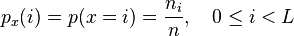
    L being the total number of gray levels in the image, n being the total number of pixels in the image, and being in fact the image's histogram for pixel value i, normalized to [0,1].

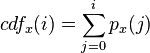
    Let us also define the cumulative distribution function corresponding to p_x as

,

which is also the image's accumulated normalized histogram.

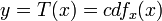
     We would like to create a transformation of the form y = T(x) to produce a new image {y}, such that its CDF will be linearized across the value range, i.e.

    for some constant K. The properties of the CDF allow us to perform such a transform (see Cumulative distribution function#Inverse); it is defined as

     Notice that the T maps the levels into the range [0,1]. In order to map the values back into their original range, the following simple transformation needs to be applied on the result:

Histogram equalization of color images

      The above describes histogram equalization on a grayscale image. However it can also be used on color images by applying the same method separately to the Red, Green and Blue components of the RGB color values of the image. However, applying the same method on the Red, Green, and Blue components of an RGB image may yield dramatic changes in the image's color balance since the relative distributions of the color channels change as a result of applying the algorithm. However, if the image is first converted to another color space, Lab color space, or HSL/HSV color space in particular, then the algorithm can be applied to the luminance or value channel without resulting in changes to the hue and saturation of the image ^[3]. There are several histogram equalization methods in 3D space. Trahanias and Venetsanopoulos applied histogram equalization in 3D color space^[4] However, it results in “whitening” where the probability of bright pixels are higher than that of dark ones ^[5]. Han et al. proposed to use a new cdf defined by the iso-luminance plane, which results in uniform gray distribution ^[6].

Examples

Small image

The following is the same 8x8 subimage as used in JPEG. The 8-bit greyscale image shown has the following values:

The histogram for this image is shown in the following table. Pixel values that have a zero count are excluded for the sake of brevity.

The cumulative distribution function (cdf) is shown below. Again, pixel values that do not contribute to an increase in the cdf are excluded for brevity.

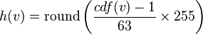
       This cdf shows that the minimum value in the subimage is 52 and the maximum value is 154. The cdf of 64 for value 154 coincides with the number of pixels in the image. The cdf must be normalized to . The general histogram equalization formula is:

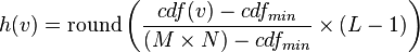
Where cdf_min is the minimum value of the cumulative distribution function (in this case 1), M × N gives the image's number of pixels (for the example above 64, where M is width and N the height) and L is the number of grey levels used (in most cases, like this one, 256). The equalization formula for this particular example is:

For example, the cdf of 78 is 46. (The value of 78 is used in the bottom row of the 7th column.) The normalized value becomes

Once this is done then the values of the equalized image are directly taken from the normalized cdf to yield the equalized values:

Notice that the minimum value (52) is now 0 and the maximum value (154) is now 255.