K均值聚类

最新推荐文章于 2021-08-09 01:35:56 发布

weixin_33708432

最新推荐文章于 2021-08-09 01:35:56 发布

阅读量619

点赞数

文章标签：数据结构与算法 python 人工智能

原文链接：https://my.oschina.net/u/1785519/blog/1564391

版权

2019独角兽企业重金招聘Python工程师标准>>>

K均值(k-means)算法

a、选择 K 个中心点(随机选择 K 行)

b、把每个数据点分配到离它最近的中心点

c、重新计算每类中的点到类中心距离的平均值（也就是说，得到长度为 p 的 均值向量，这里的 p 是变量的个数）

d、分配每个数据点到它的最近的中心点

f、重复步骤(c)和(d)直到所有的观测值不再分配或是达到最大的迭代次数（R把10次作为默认的迭代次数）

在 R 中把观测值分成 k 组并使得观测值到指定的聚类中心的平方的总和为最小，也就是说在步骤(b)和(d)中，每个观测值被分配到使下式得到最小值的那一类中：

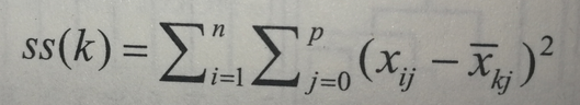
：表示第 i 个观测值中第 j 个变量的值

：表示第 k 个类中第 j 个变量的均值，其中 p 是变量的个数

kmeans(x，centers)

K均值的函数格式

 kmeans(x,centers)

x：表示数值的数据集（矩阵或数据框）

centers：要提取的聚类数目

a、函数返回类的成员、类中心、平方和（类内平方和、类间平方和、总平方和）和类大小。

b、K均值距聚类能出处理比层次聚类更大的数据集，观测值不会永远被分到一类中。均值的使用意味着所有的内变量必须是连续的，并且这个方法很有可能被异常值影响。它在非凸聚类（例如 U型）情况下会变的很差

c、由于 K 均值聚类在开始要随机选择 k 个中心点，在每次调用函数时可能获得不同的方案。使用 set.seed()函数可以保证结果是可复制的。此外，聚类方法对初始中心值的选择也很敏感。kmeans()函数有一个nstart选项尝试多种初始配置并输出最好的一个。例如，加上 nstart =25 会生成25个初始配置，通常推荐使用这种方法

d、不像层次聚类方法，K均值要求事先确定要提取的聚类个数，同样， NbClust 包可以作为参考，另外，在 K 均值聚类，类中总的平方值对聚类数量的曲线可能有帮助，可以根据图中的弯曲（类似与主成分分析中判断成分个数）选择适当的类型数量

wssplot <- function(data, nc=15, seed=1234){    #  data是用来做分析的数据值，nc是要考虑的最大聚类个数 seed是一个随机数种子
  wss <- (nrow(data)-1)*sum(apply(data,2,var))
  for (i in 2:nc){
    set.seed(seed)
    wss[i] <- sum(kmeans(data, centers=i)$withinss)}
  plot(1:nc, wss, type="b", xlab="Number of Clusters",
       ylab="Within groups sum of squares")}

葡萄酒数据的 K均值聚类

> data(wine,package = "rattle")  #从包中导入数据
> head(wine)
  Type Alcohol Malic  Ash Alcalinity Magnesium Phenols Flavanoids Nonflavanoids Proanthocyanins Color  Hue Dilution Proline
1    1   14.23  1.71 2.43       15.6       127    2.80       3.06          0.28            2.29  5.64 1.04     3.92    1065
2    1   13.20  1.78 2.14       11.2       100    2.65       2.76          0.26            1.28  4.38 1.05     3.40    1050
3    1   13.16  2.36 2.67       18.6       101    2.80       3.24          0.30            2.81  5.68 1.03     3.17    1185
4    1   14.37  1.95 2.50       16.8       113    3.85       3.49          0.24            2.18  7.80 0.86     3.45    1480
5    1   13.24  2.59 2.87       21.0       118    2.80       2.69          0.39            1.82  4.32 1.04     2.93     735
6    1   14.20  1.76 2.45       15.2       112    3.27       3.39          0.34            1.97  6.75 1.05     2.85    1450
> df <- scale(wine[-1])#-1表示剔除第一行的变量，scale()将观测值标准化

#确定聚类的个数
> wssplot(df)   #画图，有点类似碎石检验,用于确定聚类的个数，如下图1
> library(NbClust)
> set.seed(1234)
> nc <- NbClust(df,min.nc = 2,max.nc = 15,method = "kmeans")
*** : The Hubert index is a graphical method of determining the number of clusters.
                In the plot of Hubert index, we seek a significant knee that corresponds to a 
                significant increase of the value of the measure i.e the significant peak in Hubert
                index second differences plot. 
 
*** : The D index is a graphical method of determining the number of clusters. 
                In the plot of D index, we seek a significant knee (the significant peak in Dindex
                second differences plot) that corresponds to a significant increase of the value of
                the measure. 
 
******************************************************************* 
* Among all indices:                                                
* 4 proposed 2 as the best number of clusters 
* 15 proposed 3 as the best number of clusters 
* 1 proposed 10 as the best number of clusters 
* 1 proposed 12 as the best number of clusters 
* 1 proposed 14 as the best number of clusters 
* 1 proposed 15 as the best number of clusters 

                   ***** Conclusion *****                            
 
* According to the majority rule, the best number of clusters is  3 
 
 
******************************************************************* 
> par(opar)
Warning messages:
1: In par(opar) : 无法设定图形参数"cin"
2: In par(opar) : 无法设定图形参数"cra"
3: In par(opar) : 无法设定图形参数"csi"
4: In par(opar) : 无法设定图形参数"cxy"
5: In par(opar) : 无法设定图形参数"din"
6: In par(opar) : 无法设定图形参数"page"
> table(nc$Best.n[1,])

 0  1  2  3 10 12 14 15 
 2  1  4 15  1  1  1  1 
> barplot(table(nc$Best.n[1,]), xlab="Numer of Clusters", ylab="Number of Criteria",
        main="Number of Clusters Chosen by 26 Criteria")   #根据图形确定K的个数，如下图2
        
#进行 K 均值聚类分析        
> set.seed(1234)
> fit.km <- kmeans(df,3,nstart = 25) #kmeans K均值聚类分析
> fit.km$size  #分成三类，每类的观测值
[1] 51 65 62

> aggregate(wine[-1],by=list(cluster=fit.km$cluster),mean) #计算原始矩阵中每类的变量均值
  cluster  Alcohol    Malic      Ash Alcalinity Magnesium  Phenols Flavanoids Nonflavanoids Proanthocyanins    Color       Hue
1       1 13.13412 3.307255 2.417647   21.24118  98.66667 1.683922  0.8188235     0.4519608        1.145882 7.234706 0.6919608
2       2 12.25092 1.897385 2.231231   20.06308  92.73846 2.247692  2.0500000     0.3576923        1.624154 2.973077 1.0627077
3       3 13.67677 1.997903 2.466290   17.46290 107.96774 2.847581  3.0032258     0.2920968        1.922097 5.453548 1.0654839
  Dilution   Proline
1 1.696667  619.0588
2 2.803385  510.1692
3 3.163387 1100.2258

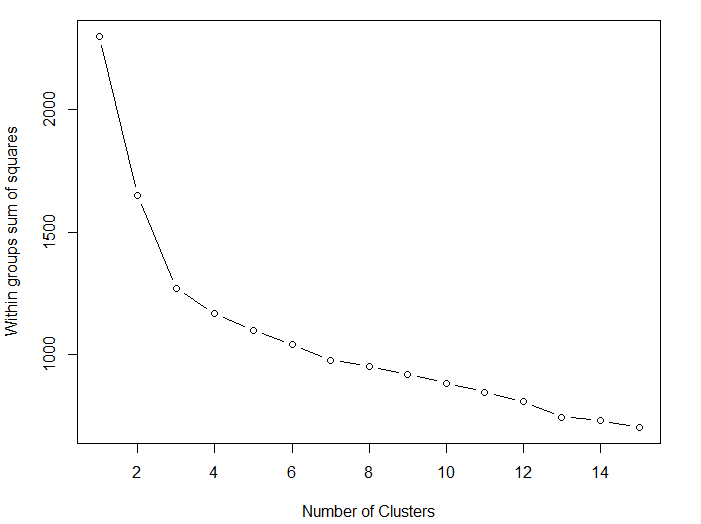
图1 画出组内的平方和和提取的聚类个数的对比。从一类到三类下降得很快（之后下降的很慢），建议选用聚类个数为 3 的解决方案

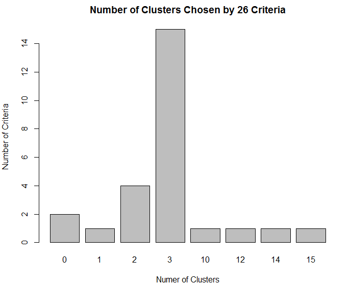
图2

K均值可以很好的揭示类型变量中的正在数据结构吗？交叉列表类型（葡萄酒品种）和类成员

> ct.km <- table(wine$Type,fit.km$cluster)
> ct.km
   
     1  2  3
  1  0  0 59
  2  3 65  3
  3 48  0  0

使用flexclust包中的兰德指数（Rand index）来量化类型变量和类之间的协议

> library(flexclust)
> randIndex(ct.km)
     ARI 
0.897495

调整的兰德指数为两种划分了一种衡量两个分区之间的协定，即调整后机会的量度，它的变化范围是从-1（不同意）到1（完全同意）。

转载于:https://my.oschina.net/u/1785519/blog/1564391

weixin_33708432

关注

0
点赞
踩
2

收藏

觉得还不错? 一键收藏
0
评论
K均值聚类

2019独角兽企业重金招聘Python工程师标准>>> ...
复制链接

扫一扫

K均值聚类

“相关推荐”对你有帮助么？