


- 正交旋转(rotate=“varimax”)
#用正交选择提取因子
> fa.varimax <- fa(correlations, nfactors=2, rotate="varimax", fm="pa")
> fa.varimax
Factor Analysis using method =  pa
Call: fa(r = correlations, nfactors = 2, rotate = "varimax", fm = "pa")
Standardized loadings (pattern matrix) based upon correlation matrix
         PA1  PA2   h2    u2 com
general 0.49 0.57 0.57 0.432 2.0
picture 0.16 0.59 0.38 0.623 1.1
blocks  0.18 0.89 0.83 0.166 1.1
maze    0.13 0.43 0.20 0.798 1.2
reading 0.93 0.20 0.91 0.089 1.1
vocab   0.80 0.23 0.69 0.313 1.2

                       PA1  PA2
SS loadings           1.83 1.75
Proportion Var        0.30 0.29
Cumulative Var        0.30 0.60
Proportion Explained  0.51 0.49
Cumulative Proportion 0.51 1.00

#后续额外内容删除
22
22
1
#用正交选择提取因子
2
> fa.varimax <- fa(correlations, nfactors=2, rotate="varimax", fm="pa")
3
> fa.varimax
4
Factor Analysis using method = pa
5
Call: fa(r = correlations, nfactors = 2, rotate = "varimax", fm = "pa")
6
Standardized loadings (pattern matrix) based upon correlation matrix
7
PA1 PA2 h2 u2 com
8
general 0.49 0.57 0.57 0.432 2.0
9
picture 0.16 0.59 0.38 0.623 1.1
10
blocks 0.18 0.89 0.83 0.166 1.1
11
maze 0.13 0.43 0.20 0.798 1.2
12
reading 0.93 0.20 0.91 0.089 1.1
13
vocab 0.80 0.23 0.69 0.313 1.2
14
15
PA1 PA2
16
SS loadings 1.83 1.75
17
Proportion Var 0.30 0.29
18
Cumulative Var 0.30 0.60
19
Proportion Explained 0.51 0.49
20
Cumulative Proportion 0.51 1.00
21
22
#后续额外内容删除
reading、vocab在第一个因子上载荷较大,picture、blocks、maze在第二因子上载荷较大,
但是general(意思为非语言的普通智力测试)在两个因子上载荷较为平均,
说明存在一个语言智力因子和一个非语言智力因子
- 斜交转轴法(rotate=“promax”)
> fa.promax <- fa(correlations, nfactors=2, rotate="promax", fm="pa")
> fa.promax
Factor Analysis using method =  pa
Call: fa(r = correlations, nfactors = 2, rotate = "promax", fm = "pa")

 Warning: A Heywood case was detected.
Standardized loadings (pattern matrix) based upon correlation matrix
          PA1   PA2   h2    u2 com
general  0.37  0.48 0.57 0.432 1.9
picture -0.03  0.63 0.38 0.623 1.0
blocks  -0.10  0.97 0.83 0.166 1.0
maze     0.00  0.45 0.20 0.798 1.0
reading  1.00 -0.09 0.91 0.089 1.0
vocab    0.84 -0.01 0.69 0.313 1.0

                       PA1  PA2
SS loadings           1.83 1.75
Proportion Var        0.30 0.29
Cumulative Var        0.30 0.60
Proportion Explained  0.51 0.49
Cumulative Proportion 0.51 1.00

 With factor correlations of
     PA1  PA2  #注意这里得到的是因子模式矩阵,而非相关系数矩阵
PA1 1.00 0.55
PA2 0.55 1.00
#删除额外的内容
27
27
1
> fa.promax <- fa(correlations, nfactors=2, rotate="promax", fm="pa")
2
> fa.promax
3
Factor Analysis using method = pa
4
Call: fa(r = correlations, nfactors = 2, rotate = "promax", fm = "pa")
5
6
Warning: A Heywood case was detected.
7
Standardized loadings (pattern matrix) based upon correlation matrix
8
PA1 PA2 h2 u2 com
9
general 0.37 0.48 0.57 0.432 1.9
10
picture -0.03 0.63 0.38 0.623 1.0
11
blocks -0.10 0.97 0.83 0.166 1.0
12
maze 0.00 0.45 0.20 0.798 1.0
13
reading 1.00 -0.09 0.91 0.089 1.0
14
vocab 0.84 -0.01 0.69 0.313 1.0
15
16
PA1 PA2
17
SS loadings 1.83 1.75
18
Proportion Var 0.30 0.29
19
Cumulative Var 0.30 0.60
20
Proportion Explained 0.51 0.49
21
Cumulative Proportion 0.51 1.00
22
23
With factor correlations of
24
PA1 PA2 #注意这里得到的是因子模式矩阵,而非相关系数矩阵
25
PA1 1.00 0.55
26
PA2 0.55 1.00
27
#删除额外的内容
对于正交旋转,因子分析的重点在于因子结构矩阵(变量与因子的相关系数),
而斜交旋转,因子分析会考虑三个矩阵
a、因子模式矩阵
即标准化的回归系数矩阵,它列出了因子预测变量的权重。
b、因子关联矩阵
即因子相关系数矩阵
c、因子结构矩阵(因子载荷阵)
因子关联矩阵显示两个因子的相关系数为0.57,相关性很大,如果因子间的关联性很低,你可能需要重新使用正交旋转来简化问题
因子结构矩阵(或称因子载荷阵)没有被列来,但 看使用公式 F = P*Phi 很庆松地得到它,其中 F 是因子载荷阵, P 为因子模式矩阵,Phi 为因子关联矩阵。下面的函数即可进行该算法
> fsm <- function(oblique){
   if (class(oblique)[2]=="fa" & is.null(oblique$Phi)){
     warning("Object doesn't")
   } else{
       P <- unclass(oblique$loading)
       F <- P %*% oblique$Phi
       colnames(F) <- c("PA1","CP2")
       return(F)
   }
 }

> fsm(fa.promax)#将参数
            PA1   PA2
general    0.64  0.69
picture    0.33  0.61
blocks     0.44  0.91
maze       0.25  0.45
reading    0.95  0.47
vocab      0.83  0.46
x
20
1
> fsm <- function(oblique){
2
if (class(oblique)[2]=="fa" & is.null(oblique$Phi)){
3
warning("Object doesn't")
4
} else{
5
P <- unclass(oblique$loading)
6
F <- P %*% oblique$Phi
7
colnames(F) <- c("PA1","CP2")
8
return(F)
9
}
10
}
11
12
> fsm(fa.promax)#将参数
13
PA1 PA2
14
general 0.64 0.69
15
picture 0.33 0.61
16
blocks 0.44 0.91
17
maze 0.25 0.45
18
reading 0.95 0.47
19
vocab 0.83 0.46
20
现在你可以看到变量与因子间的相关系数,将他们与正交选择所得因子载荷阵相比,会发现该载荷阵列的噪音比较大,这是因为允许潜在因子相关,虽然斜交方法更为复杂,但模型将更符合真实数据。
使用 factor.plot() 或者 fa.diagram() 函数,你可以绘制正交或者斜交的结果图形。来看一下代码
factor.plot(fa.promax,labels = rownames(fa.promax$loadings)) #如下图
#如下图
1
factor.plot(fa.promax,labels = rownames(fa.promax$loadings)) #如下图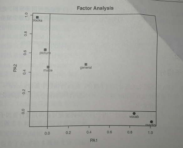
数据集 ability.cov 中心理学测验的两因子图形。词汇和阅读在第一个因子 (PA1) 上载荷较大,而积木图案、画图和迷宫在第二个因子(PA2)上载荷较大。普通智力测试在两个因子上较为平均。
使用如下代码
fa.diagram(fa.promax,simple = FLASE) #如下图,这类图形在多个因子时十分实用
这类图形在多个因子时十分实用
1
fa.diagram(fa.promax,simple = FLASE) #如下图,这类图形在多个因子时十分实用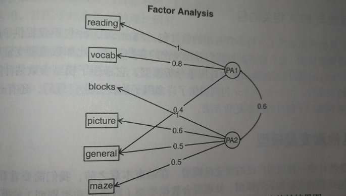
数据集 ability.cov 中心理学测验的两个因子斜交选择结果
若使 simple = TRUE ,那么将仅显示每个因子下最大的载荷,以及因子间相关系数。


 6659
6659

 被折叠的 条评论
为什么被折叠?
被折叠的 条评论
为什么被折叠?
 到【灌水乐园】发言


