Whitening transformation（白化变换）

最新推荐文章于 2024-03-26 10:05:44 发布

weixin_33860147

最新推荐文章于 2024-03-26 10:05:44 发布

阅读量804

点赞数

CC 4.0 BY-SA版权

原文链接：http://www.cnblogs.com/kevinGaoblog/archive/2012/06/20/2556335.html

(from: wikipedia)

The whitening transformation is a decorrelation method which transforms a set of random variables having the covariance matrix $Σ$ into a set of new random variables whose covariance is aI, where a is a constant and I is the identity matrix. The new random variables are uncorrelated and all have variance 1. The method is called "whitening" because it transforms the input matrix to the form of white noise, which by definition is uncorrelated and has uniform variance. It differs from decorrelation in that the variances are made to be equal, rather than merely making the covariances zero. That is, where decorrelation results in a diagonal covariance matrix, whitening produces a scalar multiple of the identity matrix.

Definition

Define $X$ to be a random vector with covariance matrix $Σ$ and mean 0. The matrix $Σ$ can be written as the outer product of $X$ and $X T$ :

$\Sigma = \operatorname{E}[XX^T]$

(注，我初一看以为写错了，按我的想法好像写成 E[X_iX_j] 更靠谱，我又想了想，后来明白了，E[X_iX_j]这样写的话，括号里面成了两个变量，而实际应该是一个变量（总体），前后可以是两个变量样本值。所以 E[XX^T]这样写是有道理的，只是注意不要误解吧。还可以这样写 E[XY^T]，X和Y是同分布，但是这是表示两个一般变量协方差的常用方法，显然和这里X是向量的环境不符合。)

Define $Σ 1/2$ as

$\Sigma^{1/2}(\Sigma^{1/2})^T = \Sigma$

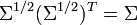
Define the new random vector $Y = Σ -1/2 X$ . The covariance of Y is

$\begin{align} \operatorname{Cov}(Y) &= \operatorname{E}[YY^T] \\ &= \operatorname{E}[(\Sigma^{-1/2}X)(\Sigma^{-1/2}X)^T] \\ &= \operatorname{E}[(\Sigma^{-1/2}X)(X^T\Sigma^{-1/2})] \\ &= \Sigma^{-1/2}\operatorname{E}[XX^T]\Sigma^{-1/2} \\ &= \Sigma^{-1/2}\Sigma\Sigma^{-1/2} \\ &= I \end{align}$

Thus, Y is a white random vector.

Based on the fact that the covariance matrix is always positive semi-definite, $Σ 1/2$ can be derived using eigenvalue decomposition:

$\Sigma\Phi = \Phi\Lambda$

$\Sigma = \Phi\Lambda\Phi^T$

$\Sigma^{1/2} = \Phi\Lambda^{1/2}$

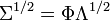
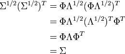
Where the matrix $Λ 1/2$ is a diagonal matrix with each element being square root of the corresponding element in $Λ$ . To show that this equation follows from the prior one, multiply by the transpose:

$\begin{align} \Sigma^{1/2}(\Sigma^{1/2})^T &= \Phi\Lambda^{1/2}(\Phi\Lambda^{1/2})^T \\ &= \Phi\Lambda^{1/2}(\Lambda^{1/2})^T\Phi^T \\ &= \Phi\Lambda\Phi^T \\ &= \Sigma \\ \end{align}$