


目录
1.白化的目的
通常,数据集的各个attributes是存在一定相关性的,这就意味着存在冗余信息。白化是一种线性变换,用于对源信号进行去相关,是一种重要的预处理过程,其目的就是降低输入数据的冗余性,使得经过白化处理的输入数据具有如下性质:
- 消除了特征之间的相关性
- 所有特征的方差都为 1
2.白化步骤
白化比其他预处理要复杂一些,它涉及以下步骤:
- 零中心数据
- 数据解相关
- 重新缩放数据
2.1 零中心数据(数据预处理)
 平均归一化
平均归一化
平均归一化指的是对数据进行减去平均值以达到中心化的目的

其中X'是标准化数据集,X是原始数据集,x̅是X的平均值。均值归一化具有将数据居中于0的效果。
标准化或归一化
标准化用于将所有特征放在相同的比例上。

其中X'是标准化的数据集,X是原始数据集, 是平均值, 并且σ是标准偏差。
2.2 数据去相关
什么是去相关呢。
即原始数据存在一定的相关性,我们想要旋转数据以使得数据不在存在相关性

那么我们要怎样旋转才能得到不想关的数据呢,实际上,在协方差矩阵中,其特征向量指示的就是数据扩散的最大方向。
因此,我们可以通过使用特征向量投影来解相关数据。这将具有应用所需旋转并移除尺寸之间的相关性的效果。以下是步骤:
- 计算协方差矩阵
- 计算协方差矩阵的特征向量
- 将特征向量矩阵应用于数据 - 这将应用于旋转
计算协方差矩阵
我们知道协方差公式如下。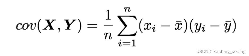
而对弈已经进行好零中心数据处理的数据中,我们已经对数据进行了去均值处理,所以都=0。
对于我们的样本X矩阵来说,其协方差矩阵就等于X和它的转置之间的点积。

计算特征向量
A为n阶矩阵,若数λ和n维非0列向量x满足Ax=λx,那么数λ称为A的特征值,x称为A的对应于特征值λ的特征向量。式Ax=λx也可写成( A-λE)x=0,并且|λE-A|叫做A 的特征多项式。当特征多项式等于0的时候,称为A的特征方程,特征方程是一个齐次线性方程组,求解特征值的过程其实就是求解特征方程的解。
对协方差矩阵 进行特征值分解,有
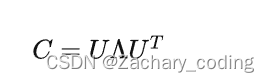
显然, 是由
的特征向量作为列向量构成的矩阵,
是对角矩阵,对角线元素为特征值。
将特征向量矩阵应用于数据
对于任一样本,其去相关后的数据y表示为

2.3 缩放处理
要求是每个输入特征具有单位方差,以直接使用

来缩放我们的去相关数据。

有时一些特征值

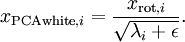
当x在区间 [-1,1] 上时, 一般取值为

上述结果即为PCA白化的结果
3.ZCA白化
ZCA 白化的全称是 Zero-phase Component Analysis Whitening。我对【零相位】的理解就是,相对于原来的空间(坐标系),白化后的数据并没有发生旋转(坐标变换)。
算法过程
ZCA白化则是在PCA白化基础上,将PCA白化后的数据旋转回到原来的特征空间,这样可以使得变换后的数据更加接近原始输入数据。 ZCA白化的计算公式:

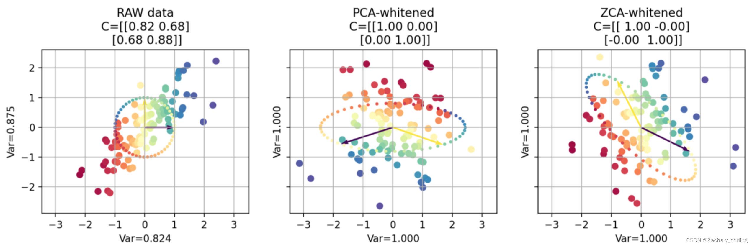
4.PCA白化和ZCA白化的区别
PCA白化ZCA白化都降低了特征之间相关性较低,同时使得所有特征具有相同的方差。
1. PCA白化需要保证数据各维度的方差为1,ZCA白化只需保证方差相等。
2. PCA白化可进行降维也可以去相关性,而ZCA白化主要用于去相关性另外。
3. ZCA白化相比于PCA白化使得处理后的数据更加的接近原始数据。
参考博客:dimensionality reduction - What is the difference between ZCA whitening and PCA whitening? - Cross Validated (stackexchange.com)白化变换:PCA白化、ZCA白化 - 知乎 (zhihu.com)


 2543
2543


 被折叠的 条评论
为什么被折叠?
被折叠的 条评论
为什么被折叠?
 到【灌水乐园】发言


