卷积神经网络最后的结果_使用卷积神经网络（CNN）对手写数字数据集mnist进行识别的结果与代码实现...

最新推荐文章于 2023-09-16 22:54:36 发布

放养的灵魂

最新推荐文章于 2023-09-16 22:54:36 发布

阅读量860

点赞数 1

文章标签：卷积神经网络最后的结果

本文链接：https://blog.csdn.net/weixin_35282313/article/details/113490493

版权

结果如下，准确率目前最高可以达到99.32%，应该还可以继续提高，提高会继续更新。

示例代码：

首先导入所需的模块

import time
from keras.datasets import mnist
from keras.utils import np_utils
import numpy as np
import pandas as pd
import matplotlib.pyplot as plt 
np.random.seed(10)

加载手写数据，如果电脑里没有数据集的话，会自动从服务器上下载，但是服务器在国外，所以速度会比较慢

(x_Train, y_Train), (x_Test, y_Test) = mnist.load_data()

为了对mnist数据集更加了解，统计多维数组所有元素出现次数

np.bincount(y_Test)

结果如下，array中的数字表示从0到9出现的次数。

array([ 980, 1135, 1032, 1010,  982,  892,  958, 1028,  974, 1009],
      dtype=int64)

#画出测试集的0~9柱形图

rects = plt.bar(range(len(np.bincount(y_Test))), np.bincount(y_Test),fc='b')  
for rect in rects:  
    height = rect.get_height()  
    plt.text(rect.get_x() + rect.get_width() / 2, height, str(height), ha='center', va='bottom')  
plt.show()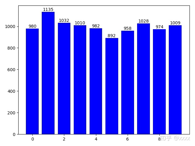

将featrues（数字图像特征）转换为四维矩阵。60000x28x28x1

x_Train4D=x_Train.reshape(x_Train.shape[0],28,28,1).astype('float32')
x_Test4D=x_Test.reshape(x_Test.shape[0],28,28,1).astype('float32')

归一化featyres数据与标签One-Hot Encoding转换

x_Train4D_normalize = x_Train4D / 255
x_Test4D_normalize = x_Test4D / 255

y_TrainOneHot = np_utils.to_categorical(y_Train)
y_TestOneHot = np_utils.to_categorical(y_Test)

接下来建立卷积神经网络模型，导入所需的模块

from keras.models import Sequential
from keras.layers import Dense,Dropout,Flatten,Conv2D,MaxPooling2D

建立Keras的模型称 “model”，后续用model.add()的方法，卷积神经网络的各个层加入到模型中

model = Sequential()

model.add(Conv2D(filters=16,
                 kernel_size=(5,5),
                 padding='same',
                 input_shape=(28,28,1), 
                 activation='relu'))

""" 建立池化层1
参数pool_size=(2, 2)，执行第1次缩减采样，将16个28x28的图像缩小为16个14x14的图像
"""
model.add(MaxPooling2D(pool_size=(2, 2)))

""" 建立卷积层2
执行第2次卷积运算，将原来的16个滤镜变为36个滤镜，input_shape=14x14的36个图像
"""
model.add(Conv2D(filters=36,
                 kernel_size=(5,5),
                 padding='same',
                 activation='relu'))

""" 建立池化层2
参数pool_size=(2, 2)，执行第2次缩减采样，将36个14x14的图像缩小为36个7x7的图像
"""
model.add(MaxPooling2D(pool_size=(2, 2)))

#加入Dropout功能避免过度拟合
model.add(Dropout(0.25))

"""  建立平坦层 
36*7*7 = 1764个神经元
"""
model.add(Flatten()) 

"""  建立隐藏层 """
model.add(Dense(128, activation='relu'))

#加入Dropout功能避免过度拟合
model.add(Dropout(0.5))

"""  建立输出层 """
model.add(Dense(10,activation='softmax'))

查看模型摘要

print(model.summary())

各个阶段的参数个数和总的参数个数都可以从中看到

_________________________________________________________________
Layer (type)                 Output Shape              Param #   
=================================================================
conv2d_1 (Conv2D)            (None, 28, 28, 16)        416       
_________________________________________________________________
max_pooling2d_1 (MaxPooling2 (None, 14, 14, 16)        0         
_________________________________________________________________
conv2d_2 (Conv2D)            (None, 14, 14, 36)        14436     
_________________________________________________________________
max_pooling2d_2 (MaxPooling2 (None, 7, 7, 36)          0         
_________________________________________________________________
dropout_1 (Dropout)          (None, 7, 7, 36)          0         
_________________________________________________________________
flatten_1 (Flatten)          (None, 1764)              0         
_________________________________________________________________
dense_1 (Dense)              (None, 128)               225920    
_________________________________________________________________
dropout_2 (Dropout)          (None, 128)               0         
_________________________________________________________________
dense_2 (Dense)              (None, 10)                1290      
=================================================================
Total params: 242,062
Trainable params: 242,062
Non-trainable params: 0
_________________________________________________________________
None

训练模型

model.compile(loss='categorical_crossentropy',
              optimizer='adam',metrics=['accuracy'])

开始执行10个训练周期 epochs=10

t1=time.time()
train_history=model.fit(x=x_Train4D_normalize, 
                        y=y_TrainOneHot,validation_split=0.2, 
                        epochs=10, batch_size=300,verbose=2)
t2=time.time()
CNNfit = float(t2-t1)
print("Time taken: {} seconds".format(CNNfit))

结果如下：

Train on 48000 samples, validate on 12000 samples
Epoch 1/10
2019-03-25 19:55:06.320701: I tensorflow/core/common_runtime/gpu/gpu_device.cc:1432] Found device 0 with properties: 
name: GeForce GTX 950M major: 5 minor: 0 memoryClockRate(GHz): 1.124
pciBusID: 0000:01:00.0
totalMemory: 2.00GiB freeMemory: 1.64GiB
2019-03-25 19:55:06.335858: I tensorflow/core/common_runtime/gpu/gpu_device.cc:1511] Adding visible gpu devices: 0
2019-03-25 19:55:19.677015: I tensorflow/core/common_runtime/gpu/gpu_device.cc:982] Device interconnect StreamExecutor with strength 1 edge matrix:
2019-03-25 19:55:19.677434: I tensorflow/core/common_runtime/gpu/gpu_device.cc:988]      0 
2019-03-25 19:55:19.677687: I tensorflow/core/common_runtime/gpu/gpu_device.cc:1001] 0:   N 
2019-03-25 19:55:19.742882: I tensorflow/core/common_runtime/gpu/gpu_device.cc:1115] Created TensorFlow device (/job:localhost/replica:0/task:0/device:GPU:0 with 1395 MB memory) -> physical GPU (device: 0, name: GeForce GTX 950M, pci bus id: 0000:01:00.0, compute capability: 5.0)
 - 33s - loss: 0.4897 - acc: 0.8478 - val_loss: 0.0961 - val_acc: 0.9726
Epoch 2/10
 - 6s - loss: 0.1406 - acc: 0.9586 - val_loss: 0.0632 - val_acc: 0.9801
Epoch 3/10
 - 6s - loss: 0.1022 - acc: 0.9693 - val_loss: 0.0521 - val_acc: 0.9832
Epoch 4/10
 - 6s - loss: 0.0829 - acc: 0.9756 - val_loss: 0.0456 - val_acc: 0.9861
Epoch 5/10
 - 6s - loss: 0.0706 - acc: 0.9779 - val_loss: 0.0396 - val_acc: 0.9878
Epoch 6/10
 - 6s - loss: 0.0632 - acc: 0.9811 - val_loss: 0.0397 - val_acc: 0.9879
Epoch 7/10
 - 6s - loss: 0.0559 - acc: 0.9827 - val_loss: 0.0445 - val_acc: 0.9870
Epoch 8/10
 - 6s - loss: 0.0513 - acc: 0.9841 - val_loss: 0.0335 - val_acc: 0.9900
Epoch 9/10
 - 6s - loss: 0.0450 - acc: 0.9861 - val_loss: 0.0338 - val_acc: 0.9906
Epoch 10/10
 - 6s - loss: 0.0419 - acc: 0.9875 - val_loss: 0.0337 - val_acc: 0.9901
Time taken: 89.0451385974884 seconds

对准确率与误差进行可视化

import matplotlib.pyplot as plt
def show_train_history(train_acc,test_acc):
    plt.plot(train_history.history[train_acc])
    plt.plot(train_history.history[test_acc])
    plt.title('Train History')
    plt.ylabel('Accuracy')
    plt.xlabel('Epoch')
    plt.legend(['train', 'test'], loc='upper left')
    plt.show()

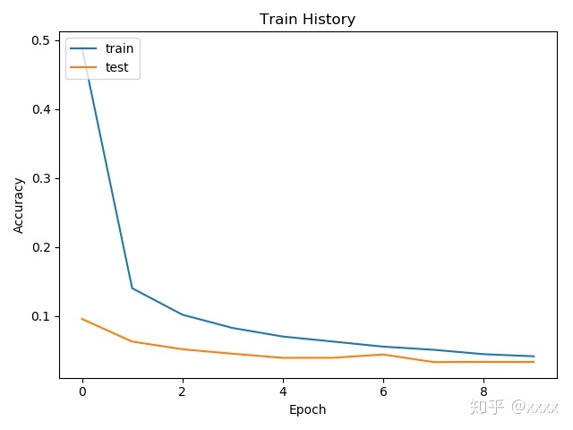
show_train_history('acc','val_acc')

show_train_history('loss','val_loss')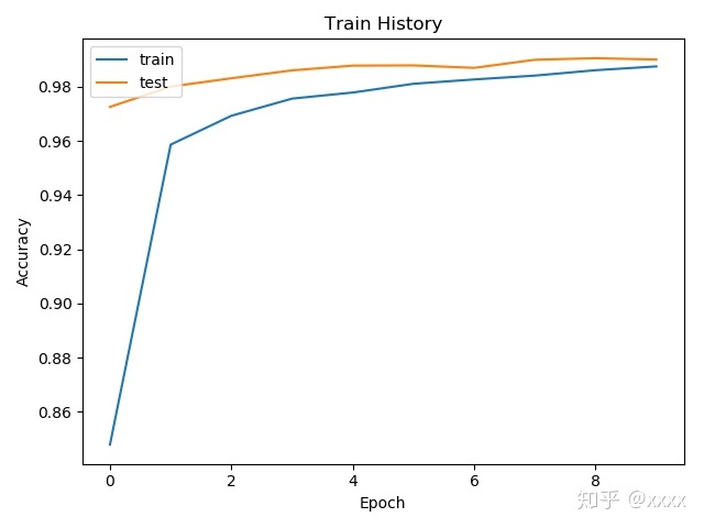

评估模型的准确率

scores = model.evaluate(x_Test4D_normalize , y_TestOneHot)
print("accuracy=", scores[1])

结果如下（结果会有略微差异），本次准确率达到99.2%。

   32/10000 [..............................] - ETA: 1:32
  448/10000 [>.............................] - ETA: 7s  
  896/10000 [=>............................] - ETA: 4s
 1248/10000 [==>...........................] - ETA: 3s
 1632/10000 [===>..........................] - ETA: 2s
 2112/10000 [=====>........................] - ETA: 2s
 2624/10000 [======>.......................] - ETA: 1s
 3136/10000 [========>.....................] - ETA: 1s
 3648/10000 [=========>....................] - ETA: 1s
 4128/10000 [===========>..................] - ETA: 1s
 4640/10000 [============>.................] - ETA: 0s
 5120/10000 [==============>...............] - ETA: 0s
 5600/10000 [===============>..............] - ETA: 0s
 6112/10000 [=================>............] - ETA: 0s
 6624/10000 [==================>...........] - ETA: 0s
 7040/10000 [====================>.........] - ETA: 0s
 7520/10000 [=====================>........] - ETA: 0s
 7968/10000 [======================>.......] - ETA: 0s
 8448/10000 [========================>.....] - ETA: 0s
 8960/10000 [=========================>....] - ETA: 0s
 9472/10000 [===========================>..] - ETA: 0s
 9920/10000 [============================>.] - ETA: 0s
10000/10000 [==============================] - 1s 142us/step
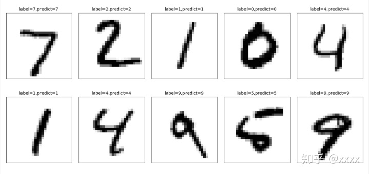
accuracy= 0.992

对测试集预测结果

prediction=model.predict_classes(x_Test4D_normalize)
prediction[:10]

结果如下：

array([7, 2, 1, 0, 4, 1, 4, 9, 5, 9], dtype=int64)

查看预测结果

def plot_images_labels_prediction(images,labels,prediction,idx,num=10):
    fig = plt.gcf()
    fig.set_size_inches(12, 14)
    if num>25: num=25 
    for i in range(0, num):
        ax=plt.subplot(5,5, 1+i)
        ax.imshow(images[idx], cmap='binary')

        ax.set_title("label=" +str(labels[idx])+
                     ",predict="+str(prediction[idx])
                     ,fontsize=10) 
        
        ax.set_xticks([]);ax.set_yticks([])        
        idx+=1 
    plt.show()

plot_images_labels_prediction(x_Test,y_Test,prediction,idx=0)

建立混淆矩阵

import pandas as pd
pd.crosstab(y_Test,prediction,
            rownames=['label'],colnames=['predict'])

结果如下：

predict    0     1     2     3    4    5    6     7    8    9
label                                                        
0        976     1     0     0    0    0    2     1    0    0
1          0  1131     1     0    0    1    1     1    0    0
2          2     0  1027     0    0    0    0     2    1    0
3          0     0     0  1002    0    3    0     3    2    0
4          0     0     0     0  977    0    1     0    1    3
5          1     0     0     4    0  884    2     0    0    1
6          4     2     0     0    2    1  949     0    0    0
7          0     1     2     1    0    0    0  1021    1    2
8          2     1     3     2    1    1    0     2  959    3
9          0     3     0     2    6    2    0     2    0  994

从混淆矩阵上看到有一个标签是5的而预测为0，查看标签是5的而预测为0的图片到底是什么样子的。

df = pd.DataFrame({'label':y_Test, 'predict':prediction})
df[(df.label==5)&(df.predict==0)]
plot_images_labels_prediction(x_Test,y_Test
                              ,prediction,idx=3558,num=1)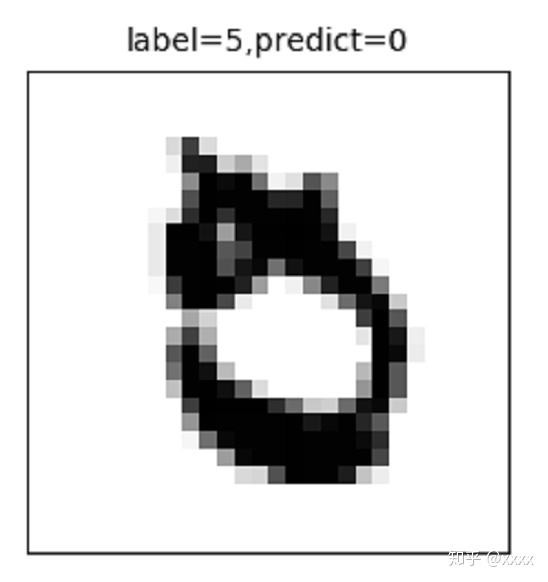

从图片上看这个5写得的确很奇怪，我自己看的话也很大可能分不出写得是5还是0。

其他的结果可以参考该代码进行修改即可。

关于SVM识别在这里

xxxx：使用支持向量机（SVM）对手写数字数据集mnist进行识别（准确率可达98.57%）zhuanlan.zhihu.com

放养的灵魂

关注

1
点赞
踩
2

收藏

觉得还不错? 一键收藏
0
评论
卷积神经网络最后的结果_使用卷积神经网络（CNN）对手写数字数据集mnist进行识别的结果与代码实现...

结果如下，准确率目前最高可以达到99.32%，应该还可以继续提高，提高会继续更新。示例代码：首先导入所需的模块import timefrom keras.datasets import mnistfrom keras.utils import np_utilsimport numpy as npimport pandas as pdimport matplotlib.pyplot as ...
复制链接

扫一扫