python 图像处理就业_python+cv环境下的图像处理

一、直方图

1.1原理

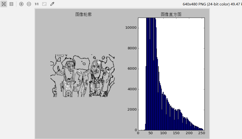
直方图是数值数据分布的精确图形表示。 这是一个连续变量的概率分布的估计，是一种条形图。为了构建直方图，第一步是将值的范围分段，即将整个值的范围分成一系列间隔，然后计算每个间隔中有多少值。 这些值通常被指定为连续的，不重叠的变量间隔。 间隔必须相邻，并且通常是(但不是必须的)相等的大小。在画图像轮廓前需要将原图像转换为灰度图像，因为轮廓需要获取每个坐标[x,y]位置的像素值。

1.2代码展示

# -*- coding: utf-8 -*-

fromPIL import Imagefrom pylab import *frommatplotlib.font_manager import FontProperties

font= FontProperties(fname=r"c:\windows\fonts\SimSun.ttc", size=14)

im= array(Image.open('C:/Users/TWZ/Desktop/kobe.jpg').convert('L')) # 打开图像，并转成灰度图像

figure()

subplot(121)

gray()

contour(im, origin='image')

axis('equal')

axis('off')

title(u'图像轮廓', fontproperties=font)

subplot(122)

hist(im.flatten(),128)

title(u'图像直方图', fontproperties=font)

plt.xlim([0,260])

plt.ylim([0,11000])

show()

1.3实验结果

二、高斯滤波及降噪

2.1原理

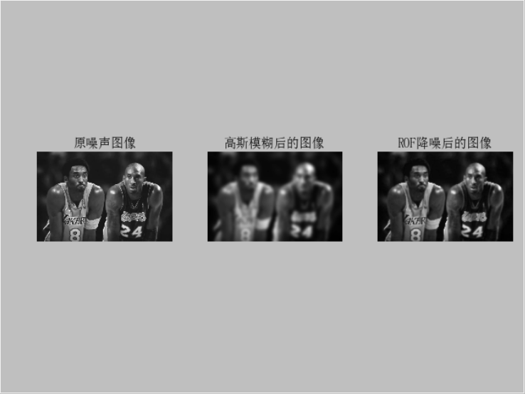
首先，高斯滤波器是一种线性滤波器，能够有效的抑制噪声，平滑图像。其作用原理和均值滤波器类似，都是取滤波器窗口内的像素的均值作为输出。其窗口模板的系数和均值滤波器不同，均值滤波器的模板系数都是相同的为1；而高斯滤波器的模板系数，则随着距离模板中心的增大而系数减小。图像降噪是一个在尽可能保持图像细节和结构信息时去除噪声的过程。

2.2代码展示

# -*- coding: utf-8 -*-

fromPIL import Imagefrom pylab import *

from numpy import *

fromnumpy import randomfromscipy.ndimage import filtersfromscipy.misc import imsavefromPCV.tools import rof"""This is the de-noising example using ROF in Section 1.5."""# 添加中文字体支持frommatplotlib.font_manager import FontProperties

font= FontProperties(fname=r"c:\windows\fonts\SimSun.ttc", size=14)

im= array(Image.open('C:/Users/TWZ/Desktop/kobe.jpg').convert('L'))

U,T=rof.denoise(im,im)

G= filters.gaussian_filter(im,10)

# save the result

#imsave('synth_original.pdf',im)

#imsave('synth_rof.pdf',U)

#imsave('synth_gaussian.pdf',G)

# plot

figure()

gray()

subplot(1,3,1)

imshow(im)

#axis('equal')

axis('off')

title(u'原噪声图像', fontproperties=font)

subplot(1,3,2)

imshow(G)

#axis('equal')

axis('off')

title(u'高斯模糊后的图像', fontproperties=font)

subplot(1,3,3)

imshow(U)

#axis('equal')

axis('off')

title(u'ROF降噪后的图像', fontproperties=font)

show()

2.3实验结果

三、直方图均衡化

3.1原理

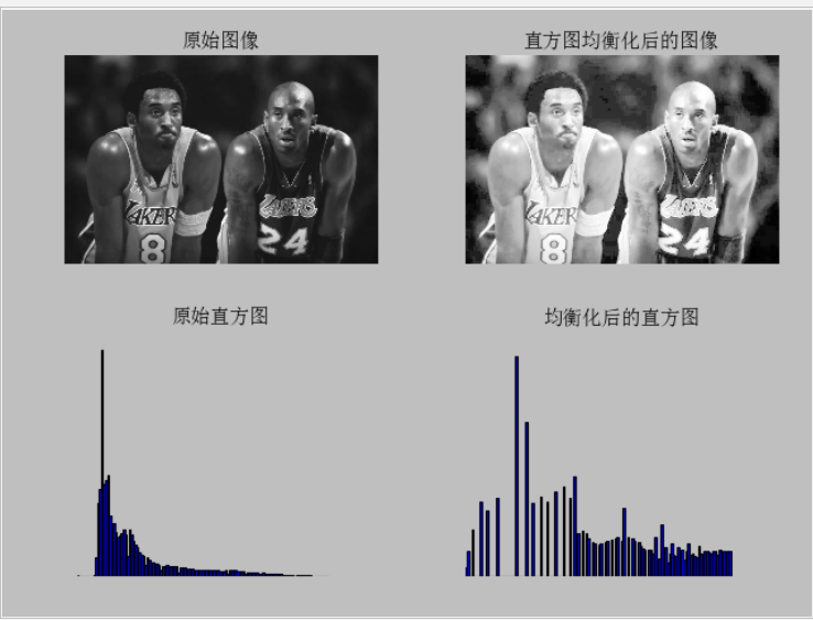
直方图均衡化实质上是对图像进行非线性拉伸,重新分配图像象元值,使一定灰度范围内象元值的数量大致相等。这样,原来直方图中间的峰顶部分对比度得到增强,而两侧的谷底部分对比度降低,输出图像的直方图是一个较平的分段直方图；如果输出数据分段值较小的话,会产生粗略分类的视觉效果。一个非常有用的例子是灰度变换后进行直方图均衡化，通过直方图均衡化可以增加图像对比度。

3.2代码展示

# -*- coding: utf-8 -*-

fromPIL import Imagefrom pylab import *

fromPCV.tools import imtoolsfrommatplotlib.font_manager import FontProperties

font= FontProperties(fname=r"c:\windows\fonts\SimSun.ttc", size=14)

im= array(Image.open('C:/Users/TWZ/Desktop/kobe.jpg').convert('L')) # 打开图像，并转成灰度图像

#im= array(Image.open('../data/AquaTermi_lowcontrast.JPG').convert('L'))

im2, cdf=imtools.histeq(im)

figure()

subplot(2, 2, 1)

axis('off')

gray()

title(u'原始图像', fontproperties=font)

imshow(im)

subplot(2, 2, 2)

axis('off')

title(u'直方图均衡化后的图像', fontproperties=font)

imshow(im2)

subplot(2, 2, 3)

axis('off')

title(u'原始直方图', fontproperties=font)

#hist(im.flatten(),128, cumulative=True, normed=True)

hist(im.flatten(),128, normed=True)

subplot(2, 2, 4)

axis('off')

title(u'均衡化后的直方图', fontproperties=font)

#hist(im2.flatten(),128, cumulative=True, normed=True)

hist(im2.flatten(),128, normed=True)

show()

3.3实验结果