可解释性机器学习

可解释性机器学习

背景

写这篇文章的背景就是可解释性机器学习在中文领域资料非常少，有一些零散的资料也不成系统，笔者根据这两个月的整理现阶段的一些可解释性的资料，可常用的代码和库，希望为大家尽一份力。文章分成，原理讲解，论文解析，代码整理，衡量特征重要性的度量四个部分。

Model-Agnostic Methods

找到所有模型都通用的检验方法，也成为post hoc interpretation。

模型解释分为两类，一类是全局的解释性（global），衡量特征在模型中起的整体作用，另一类是局部的解释性(local)，目的是对一个特定的预测条目，衡量该条样本预测分高的原因。

两类解释具有较大区别，以线性模型的解释为例，对于进行了归一化处理后的特征而言，最终的模型权重绝对值即为全局的特征重要性，因为权值越大该特征对最终分值影响越大，而对于一个取得高分的具体预测实例而言，可能在全局最重要的特征上，其分值较小，在该条样本的得分计算上并无多大贡献，因此对于线性模型单条样本的局部解释性，会使用权值乘以特征值来作为该维特征的贡献度，从而得到各个特征间的重要性排序。

Local的解释性可以通过两种方式来实现：

• 通过在一个instance的领域取点，通过简单的可解释性模型来学习complex模型的这个特定instance周边的关系。
• 用Surrogate方式。

PDP, Feature Importance, 是Global的解释方法。ICE, LIME, ALE, Anchors是local的解释方法。 Shap是既可以local又可以global。

PD & ICE

Partial Dependence和ICE通常放置在一起用，原理是对给定instance，固定除选择的特征外的其它特征值，然后对选择的特征列进行分箱迭代，每次迭代将选择的特征列全部赋予同一个值，从小到大，如果是PDP，则平均所有样本的预测值。
能展示预测值和特征之间的关系是线性的，单调性的，还是更复杂的。

For a selected predictor (x)
1. Determine grid space of j evenly spaced values across distribution of x
2: for value i in {1,...,j} of grid space do
     | set x to i for all observations
     | apply given ML model
     | estimate predicted value
     | if PDP: average predicted values across all observations
   end

def par_dep(xs, frame, model, resolution=20, bins=None):
	'''
		xs: 列名
		frame: Dataframe
		model: xgboost, lightgbm
		resolution: 分箱的精度
	'''
    pd.options.mode.chained_assignment = None
    par_dep_frame = pd.DataFrame(columns=[xs, 'partial_dependence'])    
    # 保留特定列
    col_cache = frame.loc[:, xs].copy(deep=True)  
    # 确定PD图x轴需要计算值
    if bins == None:
        min_ = frame[xs].min()
        max_ = frame[xs].max()
        by = (max_ - min_)/resolution
        bins = np.arange(min_, max_, by)  
    # 设置列为一个常数j，j按bins取值。i为总体预测的y值，j为i的均值。      
    for j in bins:
        frame.loc[:, xs] = j
        dframe = xgb.DMatrix(frame)
        par_dep_i = pd.DataFrame(model.predict(dframe))
        par_dep_j = par_dep_i.mean()[0]
        par_dep_frame = par_dep_frame.append({xs:j,
                                              'partial_dependence': par_dep_j}, 
                                              ignore_index=True)
    # 将特定列返回
    frame.loc[:, xs] = col_cache
    return par_dep_frame

ALE

主要解决特征间相互依赖问题。比如预测房子价格，特征-房间数量和特征-房子大小，比如PD会固定住房间大小，增加房间数量来画PD图，但这两个变量明显是有相关性的。ALE希望反映特征效果的相关性。通过找特征的条件分布的均值，我们平均了相似的x1值的instances的预测值。M-Plots避免平均不相似的数据的instances，但是他们混合了一个特征和其它相关特征的效果，其实就是画出两个变量的条件概率的分布。ALE通过计算预测值之间的差值，而不是求平均。比如，对于面积30m的，ALE用所有30m的例子，假装这批房子是31m和29m，用模型预测后做差。这样给了我们纯粹的面积的效果，而没有混合其它相关的特征。简单来说
，PDP和ALE都是计算了一个特征在某个格点值v时的效果。

• PDP展示的是，模型的平均预测值，在数据的instance对应想要知道的特征，都赋予选定同一个格点值v，。

• ALE是展示模型预测值在small window的变化。也就是用特征在格点值v的附近的small window的变化值。用small window的upper and lower limit of the interval来输入模型中预测后相减得到差值。
  
  

For a selected predictor (x)
1. Determine grid space of j evenly spaced values across distribution of x
2: for value i_lower, i_upper in {1,...,j} of grid space do
	   if x in (i_lower, i_upper)
	     | set x to i for all observations
	     | apply given ML model
	     | estimate difference between predicted value i_lower and i_upper
   end

Feature Interaction

通过H-statistic来衡量特征与其它特征的interaction的强度，H-statistic能够衡量根据预测结果中的特征间交互程度的方差。一般的工作流程是，先衡量interaction的强度，然后画出2D-PDP来检验interaction。
例子1: 衡量两个特征之间的Interaction程度。若两个特征之间没有interaction，则
$$P{D}_{jk}\left(x_j,x_k\right)=P{D}_j\left(x_j\right)+P{D}_k\left(x_k\right)$$
$$H_{jk}^2=\sum _{i=1}^n{\left[P{D}_{jk}\left(x_j^{(i)},x_k^{(i)}\right)-P{D}_j\left(x_j^{(i)}\right)-P{D}_k\left(x_k^{(i)}\right)\right]}^2/\sum _{i=1}^{n}P{D}_{jk}^2\left(x_j^{(i)},x_k^{(i)}\right)$$

PD指partial dependence function。

1: for variable i in {1,...,p} do
     | f(x) = estimate predicted values with original model
     | pd(x) = partial dependence of variable i
     | pd(!x) = partial dependence of all features excluding i
     | upper = sum(f(x) - pd(x) - pd(!x))
     | lower = variance(f(x))
     | rho = upper / lower
   end
5. Sort variables by descending rho (interaction strength)  

例子2:衡量一个特征与其余特征之间的Interaction程度。

$$\hat{f}(x)=P{D}_j\left(x_j\right)+P{D}_{-j}\left(x_{-j}\right)$$
$-j$表示$j$的补集。
$$H_j^2=\sum _{i=1}^n{\left[\hat{f}\left(x^{(i)}\right)-P{D}_j\left(x_j^{(i)}\right)-P{D}_{-j}\left(x_{-j}^{(i)}\right)\right]}^2/\sum _{i=1}^n{\hat{f}}^2\left(x^{(i)}\right)$$

2-way interaction strength of feature
1: i = a selected variable of interest
2: for remaining variables j in {1,...,p} do
     | pd(ij) = interaction partial dependence of variables i and j
     | pd(i) = partial dependence of variable i
     | pd(j) = partial dependence of variable j
     | upper = sum(pd(ij) - pd(i) - pd(j))
     | lower = variance(pd(ij))
     | rho = upper / lower
   end
6. Sort interaction relationship by descending rho (interaction strength)

这两个例子衡量了j没有interaction的程度。通过计算PD输出后的方差，得到interaction程度的统计量。若统计量是0意味着无interaction。若统计量是1，意味着对预测的影响，只来自于两个特征的interaction，而不来自于两个特征本身。由于计算成本大，一般采用抽样计算。

优势：

• H-statistic的理论是PD分解
• H-statistic的能够检验所有的Interactions

劣势：

• 计算成本高
• 难以判断什么时候说明interaction是强的
• 不能应用于图像分类器

Permutation Feature Importance

概念是计算模型预测的误差值，若一个特征很重要，那么shuffling这个值，预测误差值会增加。若特征不重要，shulffing之后，预测误差值不变。

优势：

• global的解释性，会考虑所有interaction的效果。
• Permutation feature importance 不要求重新训练模型。

劣势：

• 需要有true y，否则模型无法训练。
• 与模型误差率相关，无法与模型输出的方差程度联系。

For any given loss function do
1: compute loss function for original model
2: for variable i in {1,...,p} do
     | randomize values
     | apply given ML model
     | estimate loss function
     | compute feature importance (permuted loss / original loss)
   end
3. Sort variables by descending feature importance   

代码skater

from skater.core.explanations import Interpretation
interpreter = Interpretation()
interpreter.partial_dependence.plot_partial_dependence()

Global Surrogate

用简单模型替代复杂模型的方式，思路较简单。

1. apply original model and get predictions
2. choose an interpretable "white box" model (linear model, decision tree)
3. Train the interpretable model on the original dataset and its predictions
4. Measure how well the surrogate model replicates the prediction of the black box model
5. Interpret / visualize the surrogate model

Local Surrogate（LIME）

Scoped Rules (Anchors)

Anchors是LIME的改进版，也是一种local的方法，会将特征和y简化成IF-Then形式。简单来说，就是能找到特征里面的一个小子集，只要出现这个特征子集，那么这个预测结果总是相同。

$${\mathbb{E}}_{{\mathcal{D}}_x(z|A)}\left[1_{f(x)=f(z)}\right]\ge \tau ,A(x)=1$$
这个公式的意思是，在以A为条件下，在x领域分布中多次抽样z，其中抽样的z和x在模型输出后相等的期望应该大于$\tau$

以论文的例子举例：
D是原空间的分布，现在要找到Anchors，能让只要出现Anchors，则句子的情感就会预测为positive。做法是，找到了‘not’ ‘bad’两个词，在这两个词的条件概率下，重新抽样组成句子，拿重新组成的句子输入模型去预测，看新组成句子的情感正负性，使其概率最大越好。

Shapley Values

Shapley value起源于博弈论：n个人合作，创造了v(N)的价值，如何对所创造的价值进行分配。
notation: 全集N={x1,x2,⋯,xn}
有n个元素xi，任意多个人形成的子集S⊆N，有v(S)表示S子集中所包括的元素共同合作所产生的价值。最终分配的价值（Shapley Value）ψi(N,v)其实是求累加贡献（marginal contribution）的均值。例如A单独工作产生价值v({A})，后加入B之后共同产生价值v({A,B})，那么B的累加贡献为v({A,B})−v({A})。对于所有能够形成全集N的序列，求其中关于元素xi的累加贡献，然后取均值即可得到xi的Shapley Value值。但枚举所有序列可能性的方式效率不高，注意到累加贡献的计算实际为集合相减，对于同样的集合计算次数过多是效率低下的原因。公式中S表示序列中位于xi前面的元素集合，进而N∖S∖{xi}表示的是位于xi后面的元素集合，而满足只有S集合中的元素位于xi之前的序列总共有|S|!(|N|−|S|−1)!个，其内序列中产生的xi累加贡献都是v(S⋃{xi})−v(S)；最后对所有序列求和之后再取均值。
假设特征全集为F，则有：

ϕ i = ∑ S ⊆ F \ [ i } ∣ S ∣ ! ( ∣ F ∣ − ∣ S ∣ − 1 ) ! ∣ F ∣ ! [ f S ∪ { i } ( x S ∪ { i } ) − f S ( x S ) ] \phi_{i}=\sum_{S \subseteq F \backslash[i\}} \frac{|S| !(|F|-|S|-1) !}{|F| !}\left[f_{S \cup\{i\}}\left(x_{S \cup\{i\}}\right)-f_{S}\left(x_{S}\right)\right] ϕi​=S⊆F\[i}∑​∣F∣!∣S∣!(∣F∣−∣S∣−1)!​[fS∪{i}​(xS∪{i}​)−fS​(xS​)]

求得每一维特征的shapley value值，值越大对目标函数的影响越正向，值越小对目标函数的影响越负向。

ob = single observation of interest
1: for variables j in {1,...,p} do
     | m = random sample from data set
     | t = rbind(m, ob)
     | f(all) = compute predictions for t
     | f(!j) = compute predictions for t with feature j values randomized
     | diff = sum(f(all) - f(!j))
     | phi = mean(diff)
   end
2. sort phi in decreasing order

优势：

• 由于是通过预测值与平均预测值的差值进行比较所以预测是相对公平分布的

缺点：

• 运算时间过大

SHAP(SHapley Additice exPlanations)

SHAP和Shapley values的区别有两点。第一，SHAP作者提出了KernelSHAP，是一种kernel-based的评估方式对于Shapley values。并且提出了TreeSHAP，一种可以有效评估树模型的方法。第二，SHAP有很多基于集合Shapley values的全局解释的方法。

定义：SHAP的目标是通过计算每个特征的对预测的贡献值，来解释an instance的预测值。SHAP解释方法从coalitional game theory计算了Shapley values. An instance的特征值作为players在coalition

$$g\left(z^{\prime }\right)={\varphi }_0+\sum _{j=1}^M{\varphi }_j{z}_j^{\prime }$$

Shapley values 是唯一满足Efficiency, Symmetry, Dummy Additivity的特性的方法。
SHAP满足如下三种特征

• 1. Local accuracy.
• 2. Missingness. 把缺失值赋值0。
• 3. Consistency. 若模型变化，则特征值的边缘概率增加或不变。

KernelSHAP

待补充

5.10.4 Examples

随机森林分类器。SHAPE计算Shapley values的方式是一样的，但是每个特征值是一个force可以increase or decrease预测值。

这个图是SHAP值来解释两个instance的的癌症可能性。基线是0.066。第一个instance是0.6，低于基线。STD这样increasing预测值的因素，被decreasing的因素抵消。第二个instance是0.71。51的岁数和34年的吸烟历史增加了的癌症的概率。
这个图反映的是每个特征贡献于推动模型远离base value的结果。

5.10.5 SHAP Feature Importance

SHAP的Feature importance是根据特征所拥有的Shapley values值排序，计算公式是Shapley values绝对值的均值。Permutation feature importance是基于模型性能的下降，而SHAP是基于特征属性的大小。虽然有用，但是也只能显示importance。summary plot能显示更多信息。

5.10.6 SHAP Summary Plot

Summary plot结合了feature importance和feature effects。S图的每一个是一个instance的一个特征的Shapley value值。y轴是被feature value决定，x轴是被Shapley value决定。重叠在一起的点可以反映每个特征的Shapley value的分布。并且features根据importance排序。

在summary plot，能反映特征值的大小和对预测的贡献度之间的关系，但是具体的关系的形式，要通过看SHAP dependence plots

5.10.7 SHAP Dependence Plot

SHAP 特征依赖图或许是最简单的global interpretation plot，选择特征，为每一个instance在x轴画特征值，在y轴是对应的Shapley value。
$${\left\{\left(x_j^{(i)},{\varphi }_j^{(i)}\right)\right\}}_{i=1}^n$$

这幅图反映了，对比与0年，年份低降低了得癌症的概率，年份高的时候增加了得癌症的概率。
PDP和ALE展示的是平均的效果，SHAP依赖图在y轴上的展示出了方差性，特别是在interactions时，SHAP依赖图在y轴上会更加分散。

5.10.8 SHAP Interaction Values

interaction effect指的是在单个特征效果解释后的，结合的特征效果。计算方式被定义为

ϕ i , j = ∑ S ⊆ { { i , j } ∣ S ∣ ! ( M − ∣ S ∣ − 2 ) ! 2 ( M − 1 ) ! δ i j ( S ) \phi_{i, j}=\sum_{S \subseteq\{\{i, j\}} \frac{|S| !(M-|S|-2) !}{2(M-1) !} \delta_{i j}(S) ϕi,j​=S⊆{{i,j}∑​2(M−1)!∣S∣!(M−∣S∣−2)!​δij​(S)
当 $i\ne j$
δ i j ( S ) = f x ( S ∪ { i , j } ) − f x ( S ∪ { i } ) − f x ( S ∪ { j } ) + f x ( S ) \delta_{i j}(S)=f_{x}(S \cup\{i, j\})-f_{x}(S \cup\{i\})-f_{x}(S \cup\{j\})+f_{x}(S) δij​(S)=fx​(S∪{i,j})−fx​(S∪{i})−fx​(S∪{j})+fx​(S)
这个公式减去了特征的主效果，以便我们能够得到interaction effect。直接看图

这张图显示了增加了一个STD变量后的interaction效果。能看出，若年份低的时候，有STD出现，则会增加得癌症的概率。若年份高的时候，有STD出现，则会降低得癌症的概率。

Clustering SHAP values

可以通过Shapley values来聚类数据，目的是找到相似的instances，这意味着通过解释性的相似度来聚类。每个SHAP值都有同样的预测空间的单位。

每个x轴的每个位置，是一个instance。红色SHAP值提升预测，blue降低预测。
这个图是展示多个instance在一张图上，是上图的多instances。横坐标表示第i个instances的Shape value。

优势：

得到对比的解释，通过比较预测和平均预测。SHAP联系来LIME和Shapley values。SHAP能迅速实施对于tree-based models。迅速计算global model interpretation成为可能，比如feature importance, feature dependence, interactions, clustering, summary plots。并且在SHAP中，global解释与local的解释是一致的。

劣势：

KernelSHAP很慢。这使得一些feature importance的方法不可用。KernelSHAP 忽略来特征依赖性，许多扰动的方法都有这个问题。通过从随机instances提取特征值来替换特征值，会更容易从边缘分布采样。但是，如果特征间是相关的，这导致不相关的数据点上。TreeSHAP解决这个问题通过清晰的建模条件概率预测。

Example-Based Explanations

选取数据集中的特定例子，来解释model的行为和潜在的数据分布。所以这种方法与上一种方法的不同是在于，它通过选取一些instances来解释模型，而不是对特征做总结。

Counterfactuals Guided by Prototypes

人们总是考虑，我怎么样改变银行可以批准我的贷款。反例可以导致不同的输出，

论文解读

FRIEDMAN1999年论文

• Relative importance of input variables.
  对单个输入的$x_j$, Relative influences $I_j$是最有效描述模型的，在模型输出的在联合输入分布的变化程度上。数模型通过分段的常数，来近似$I_j$。
  $${\hat{I}}_j^2(T)=\sum _{t=1}^{J-1}{\hat{i}}_t^{2}1\left(v_t=j\right)$$
  $${\hat{I}}_j^2=\frac{1}{M}\sum _{m=1}^M{\hat{I}}_j^2\left(T_m\right)$$
  这个公式的意思是，先对单颗树计算j的相对重要性，再把迭代加上所有的树的相对重要性。单颗树的相对重要性的计算是，若分叉节点是由特征j分叉的，则用1*$i_t^2$，$i_t^2$是用特征j分叉后得到的信息增益。
  $$i^2\left(R_l,R_r\right)=\frac{w_l{w}_r}{w_l+w_r}{\left({\bar{y}}_l-{\bar{y}}_r\right)}^2$$
• PDP。不再解释
• Randomly generated function

蚂蚁金服2018年论文

https://www.sohu.com/a/232481440_99940985
主要关注GDBT模型各种变式，提供统一的局部解释方案，对每一个预测样本给出各个特征的贡献度，从而对模型预测结果进行归因。

对于GBDT模型全局的解释性，Freidman基于树模型中分裂点对均方误差的影响，提出了评估特征重要性的方法，并被广泛用在特征筛选和模型分析当中。然而，对于对其局部解释性则需要将特征值纳入考虑，希望能够在有解释性需求的场景，对GBDT的单条结果提供个性化的解释。

对于GDBT的局部解释性，主要问题是

第一，不同于线性模型，模型权值与各维特征一一对应，GBDT这种树形模型的权值存在于叶子结点上，一个叶子结点实际上是从根节点开始，由一系列特征分裂点、特征分裂值决定的一条路径，也就是一个叶节点上的分值是多个特征共同决定的，所以问题的难点就在于需要对单个特征的贡献度进行定义。

第二，由于GBDT模型的特点，它的每一棵树拟合的都是当前的残差，同一特征在不同的树上贡献度也是不同的，因为随着残差的逐渐减小，后面的树对最后预测分值的贡献度也是更小的，因此随机森林RF（Random Forest）模型那种基于样本标签分布变化的局部解释性方案不适用于GBDT模型。此外，GBDT还具有不同的变式，可能采用不同的损失函数和优化策略，解释性方案应该具有通用性。

方法介绍
分裂特征f落到叶节点c后的局部的特征贡献，由子节点分值(Sc)与父节点（Sp）分值的差表示
$$L{I}_f^c=\{\begin{array}{ll}{S}_c-S_p& \text{ if the split in the parent is performed over the feature }f\\ 0& \text{ otherwise }\end{array}$$
$$S_p=\frac{1}{2}\left(S_{c1}+S_{c2}\right)\to \frac{N_{c1}\times S_{c1}+N_{c2}\times S_{c2}}{N_{c1}+3I_{c2}}$$
其中Sp表示父节点的分值，Sc1、Sc2分别表示两个子节点的分值，Nc1、Nc2则对应训练集中子节点c1，c2所包含的样本数。
$$\begin{array}{c}F{C}_{i,m}^f={\sum }_{c\in \text{path}(i)}L{I}_f^c\\ F{C}_i^f={\sum }_{m=1}^{M}F{C}_{i,m}^f\end{array}$$
其中，第一步表示的是计算特征f在样本i、单棵树m上的贡献度，第二步表示在所有树上进行贡献度的累加，获得最终贡献度总计。

RF的解释方法，和GDBT的解释方法。
在路径上的features都对final prediction有贡献，对于a single tree。
评估特征的贡献度的思想是取正类分布变化值。先计算树中每个节点的正类的百分比，然后记录parent和child nodes的百分比的不同，再计算每个特征在每颗树的贡献度，平均特征在森林中的贡献度。很容易记录local的贡献度，和相对于的划分特征。
GDBT是另一种结合回归树的集合。
两点不同，第一RF是voting，GBDT是计算所有树的score和，并且是顺序计算。第二，GBDT输出是socre而不是主要的class类型。

量化模型复杂度，通过函数分解，为了更好的模型解释性

这是第一个可以衡量global interaction强度，主要复杂度，特征数量。

• NF。模型使用的特征数量。定义特征使用从改变特征值会改变预测值。
• Interaction Strength。
• Main Effect Complexity。

可解释性代码库整理

由于日后运用主要在信贷数据上，所以我主要整理的是分类问题的可解释性。
tabular explainers需要training set, 如果特征是numerical的，需要计算mean和std。如果是categorical的，需要计算每个值的出现频率。
lime:

Shap

import xgboost
import shap
# 初始化
shap.initjs()
# 训练模型
X,y = shap.datasets.boston()
model = xgboost.train({"learning_rate": 0.01}, xgboost.DMatrix(X, label=y), 100)
# 用SHAP values解释模型的预测
explainer = shap.TreeExplainer(model) # 选用树分类器
shap_values = explainer.shap_values(X) # 计算全样本的shap value
# 画图
shap.force_plot(explainer.expected_value, shap_values, X)
shap.dependence_plot("RM", shap_values, X)
shap.summary_plot(shap_values, X)
shap.summary_plot(shap_values, X, plot_type="bar")

Skater

Skater库提供Feature Importance, PDP, LIME, Surrogate几种解释性方法。分类问题用类别的概率。
Skater的Feature Importance是根据给特定的特征一个扰动，衡量预测值熵的变化程度。
Skater的LIME

# 载入数据和训练模型
from sklearn.datasets import load_breast_cancer
from sklearn.ensemble import RandomForestClassifier
import numpy as np
DATA = load_breast_cancer()
X, y, features = DATA.data, DATA.target, DATA.feature_names
rf = RandomForestClassifier()
rf.fit(X,y)

# global: FI & PDP
from skater import Interpretation # FI & PD
from skater.model import InMemoryModel
model = InMemoryModel(rf.predict_proba, examples = X) # 将X存储进内存
interpreter = Interpretation()
interpreter.load_data(X, feature_names=features)
interpreter.feature_importance.feature_importance(model) # FI
interpreter.feature_importance.plot_feature_importance(model, ascending=True) # FI
interpreter.partial_dependence.plot_partial_dependence([features[0],features[1]],model) # PDP
# local: lime
from skater.core.local_interpretation.lime.lime_tabular import LimeTabularExplainer # LIME
explainer = LimeTabularExplainer(X, mode='classification',feature_names=DATA.feature_names, class_names=DATA.target_names)
i = 1
exp = explainer.explain_instance(X[i], rf.predict_proba, num_features=2, top_labels=1) # 对于多分类问题，设置top_labels=1，可只解释第一个类。
exp.show_in_notebook(show_table=True, show_all=False)

ALIBI(整合了Anchor)

https://docs.seldon.io/projects/alibi/en/stable/overview/getting_started.html

from sklearn.datasets import load_breast_cancer
from sklearn.ensemble import RandomForestClassifier
DATA = load_breast_cancer()
X, y, features, class_names = DATA.data, DATA.target, DATA.feature_names, list(DATA.target_names)
rf = RandomForestClassifier()
rf.fit(X,y)

# Anchors
from alibi.explainers import AnchorTabular
explainer = AnchorTabular(rf.predict_proba, features)
explainer.fit(X)
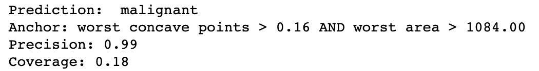
idx = 0
print('Prediction: ', class_names[explainer.predict_fn(X[idx].reshape(1, -1))[0]])
explanation = explainer.explain(X[idx], threshold=0.95)
print('Anchor: %s' % (' AND '.join(explanation['names'])))
print('Precision: %.2f' % explanation['precision'])
print('Coverage: %.2f' % explanation['coverage'])

# CEM

# Counterfactuals Guided by Prototypes

elit

elit5支持解释weights和

from sklearn.model_selection import train_test_split
from sklearn.datasets import load_breast_cancer
from sklearn.ensemble import RandomForestClassifier
DATA = load_breast_cancer()
X, y, features, class_names = DATA.data, DATA.target, DATA.feature_names, list(DATA.target_names)
X_train, X_test, y_train, y_test = train_test_split(X, y, test_size=0.33, random_state=42)
rf = RandomForestClassifier()
rf.fit(X,y)

from eli5.sklearn import PermutationImportance
from eli5 import show_prediction
from eli5 import show_weights

show_weights(rf)
show_prediction(rf,X[0],show_feature_values=True)
perm = PermutationImportance(rf).fit(X_test, y_test)
show_weights(perm)

衡量特征重要性的度量的好坏

http://www.sohu.com/a/274021299_100285715
任何好的特征归因方法应该遵循：

• 1. 一致性。每当我们更改模型以使其更依赖于某个特征时，该特征归因重要性不应该降低。
• 2. 准确性。所有特征重要性的综合应该等于模型的总重要性。
     为了检查一致性，必须定义“重要性”。两种定义：1）删除一组特征时，模型的预期准确性的变化 2）当我们删除一组特征时，模型预期输出的变化。 第一个重要性定义衡量特征对模型的全局影响，第二个定义测量特征对单个预测的个性化影响。

xgboost中的feature_importance的权重，覆盖，增益三种方法都是全局特征归因方法。但在信贷领域，还需要为每个客户提供个性化的解释。为了检查一致性，在树模型上运行五种不同的特征归因方法。

最终结果是只有Tree SHAP既一致又准确，这并非巧合。鉴于我们需要一种既一致又准确的方法，事实证明只有一种方法可以分配要素重要性。详细信息在我们最近的NIPS论文中，但总结是，博弈论中关于公平利润分配的证据导致机器学习中特征归因方法的唯一性结果。Lloyd Shapley在20世纪50年代推导出来之后，这些独特的价值被称为Shapley值。我们在这里使用的SHAP值来自与Shapley值相关的几个个性化模型解释方法的统一。Tree SHAP是一种快速算法，可以在多项式时间内精确计算树的SHAP值，而不是经典的指数运行时。

Reference

• 可解释性机器学习book
• SHAP的GITHUB
• Skater
• Anchor的GITHUB locally
• Elit的GITHUB
• Anchors论文
• Unpack Local Model Interpretation for GBDT
• 添加链接描述
• Introduction to ML Interpretability
• Quantifying Model Complexity via Functional Decomposition for Better Post-Hoc Interpretability
• https://arxiv.org/pdf/1905.03151.pdf

英文版

LIME： constructs explanations by creating a local model, like a regression model, for the instance for which an explanation is required. The data for the local model is generated by perturbing the instance of interest, observing the change in labels and using it to train a new model.
Shapley values： take a game theoretical perspective to determine the relative contribution of variables to the predictions by considering all possible combinations of variables as cooperating and competing coalitions to maximize payoff, defined in terms of the prediction

Feature importance
For any given loss function do
1: compute loss function for original model
2: for variable i in {1,...,p} do
     | randomize values
     | apply given ML model
     | estimate loss function
     | compute feature importance (permuted loss / original loss)
   end
3. Sort variables by descending feature importance

PDP&ICE
For a selected predictor (x)
4. Determine grid space of j evenly spaced values across distribution of x
2: for value i in {1,...,j} of grid space do
     | set x to i for all observations
     | apply given ML model
     | estimate predicted value
     | if PDP: average predicted values across all observations
   end

Measuring Interaction
1: for variable i in {1,...,p} do
     | f(x) = estimate predicted values with original model
     | pd(x) = partial dependence of variable i
     | pd(!x) = partial dependence of all features excluding i
     | upper = sum(f(x) - pd(x) - pd(!x))
     | lower = variance(f(x))
     | rho = upper / lower
   end
5. Sort variables by descending rho (interaction strength)  

2-way interaction strength of feature
1: i = a selected variable of interest
2: for remaining variables j in {1,...,p} do
     | pd(ij) = interaction partial dependence of variables i and j
     | pd(i) = partial dependence of variable i
     | pd(j) = partial dependence of variable j
     | upper = sum(pd(ij) - pd(i) - pd(j))
     | lower = variance(pd(ij))
     | rho = upper / lower
   end
6. Sort interaction relationship by descending rho (interaction strength)