GANSYNTH（基于对抗性神经网络的音频合成）

最新推荐文章于 2024-06-08 10:04:04 发布

芝士小奶盖

最新推荐文章于 2024-06-08 10:04:04 发布

阅读量5.1k

点赞数 6

分类专栏： AI音乐合成文章标签： GAN GANsynth 音频合成

本文链接：https://blog.csdn.net/weixin_37567451/article/details/88390205

版权

AI音乐合成专栏收录该内容

1 篇文章 0 订阅

订阅专栏

本文基于文章《Adversarial neural audio synthesis》

读了论文，看了源代码，还是有很多地方对不上，不理解（因为代码部分还是比较难的,音频音乐部分也涉及到很多信号处理方面的知识）。理解的我就补充进来。

这是谷歌团队的megenta项目，首先先了解对抗神经网络（Gan，网上一大堆，可以找个demo看一看跑一跑就懂），以及progressive Gan, progressive Gan不理解的请看谷歌团队的另一篇文章《progressive groeing of gans for improved quality,stability,and variation》,这里不详细说明。

================================================================

写之前，首先想归整几个英语单词：

note:音符

timebre:音色

pitch：音调

=================================================================

1.首先先看dataset

Dataset是基于NSynth dataset,它包含了来自1000种乐器的300000个musical notes，NSynth dataset是一个具有高度多样化的timebre和pitch组成的数据集，且具有高度结构化的pitch,velocity,instrument,acoustic qualities标签。其中每个sample都是4秒，16kHz，维度为64000，音调范围MIDI 24~84,因为这个范围人听起来最舒适。

NSynth可以下载两种格式：TFRecord格式和json格式（不太懂，不重要）

每个样本都包含以下14个特征：（浏览就行，知道是这14个特征组成的那64000维就行）

Feature	Type	Description
note	`int64`	A unique integer identifier for the note.
note_str	`bytes`	A unique string identifier for the note in the format `<instrument_str>-<pitch>-<velocity>`.
instrument	`int64`	A unique, sequential identifier for the instrument the note was synthesized from.
instrument_str	`bytes`	A unique string identifier for the instrument this note was synthesized from in the format `<instrument_family_str>-<instrument_production_str>-<instrument_name>`.
pitch	`int64`	The 0-based MIDI pitch in the range [0, 127].
velocity	`int64`	The 0-based MIDI velocity in the range [0, 127].
sample_rate	`int64`	The samples per second for the `audio` feature.
audio*	`[float]`	A list of audio samples represented as floating point values in the range [-1,1].
qualities	`[int64]`	A binary vector representing which sonic qualities are present in this note.
qualities_str	`[bytes]`	A list IDs of which qualities are present in this note selected from the sonic qualities list.
instrument_family	`int64`	The index of the instrument family this instrument is a member of.
instrument_family_str	`bytes`	The ID of the instrument family this instrument is a member of.
instrument_source	`int64`	The index of the sonic source for this instrument.
instrument_source_str	`bytes`	The ID of the sonic source for this instrument.

* Note: the “audio” feature is ommited from the JSON-encoded examples since the audio data is stored separately in WAV files keyed by the “note_str”.

其中的instrument_source是这样的（说白了就是音符乐器的声音制作方法。每个乐器（及其所有音符）都对应以下一种，就这3中声音制作方法）：

Index	ID
0	acoustic
1	electronic
2	synthetic

其中还有个instrument_family是这样的（说白了就是音符属于那种类别的乐器，每个乐器对应以下一种，一共是11种系别）：

Index	ID
0	bass
1	brass
2	flute
3	guitar
4	keyboard
5	mallet
6	organ
7	reed
8	string
9	synth_lead
10	vocal

以及Note Qualities等，后面几种类似不讲，详细请参考https://magenta.tensorflow.org/datasets/nsynth#example-features。

以上是dataset。

=========================================================================================

我们知道Gan包含了两个模块，生成模型（Generative Model）和判别模型（Discriminative Model），

•G是一个生成audio的网络,它接收一个随机的噪声z,通过这个噪声来生成audio,记做G(z)。

•D是一个判别网络,判别一个audio是不是“真实的”,它的输入参数是x,x代表一个audio,输出D(x)代表x为真实audio的概率,如果为1,就代表100%是真实的audio,而输出为0,就代表不可能是真实的audio。

在训练过程中,生成网络G的目标就是尽量生成真实的audio去欺骗判别网络D。而D的目标就是尽量把G生成的audio和真实的audio分别开来。这样,G和D构成了一个动态的“博弈过程”。

最后博弈的结果是什么?

在最理想的状态下,G可以生成足以“以假乱真”的audio G(z)。对于D来说,它难以判定G生成的audio究竟是不是真实的,因此D(G(z)) = 0.5。

这样我们的目的就达成了：我们得到了一个生成式的模型G,它可以用来生成audio。

一.首先我们来看生成模型G（完全从代码分析而来）

If:

如果给定了MIDI文件，则通过在latent向量之间插值合成音符；如果没有给定MIDI文件，则合成随机的音符。

具体怎么插值呢？我们看一下插值函数的代码：

def slerp(p0, p1, t):
  """Spherical linear interpolation."""
  omega = np.arccos(np.dot(
      np.squeeze(p0/np.linalg.norm(p0)), np.squeeze(p1/np.linalg.norm(p1))))
  so = np.sin(omega)
  return np.sin((1.0-t)*omega) / so * p0 + np.sin(t*omega)/so * p1

翻译成数学公式就是：

$\Omega =\arccos (p_{0}\cdot p_{1})$

$slerp(p_{0},p_{1},t)=\tfrac{sin[(1-t)\Omega ]}{sin\Omega }p_{0}+\tfrac{sin[t\Omega ]}{sin\Omega }p_{1}$

这其实就是球面插值：曲线上任意一点必是两个终点的线性组合，p0是起点，p1是终点，0≤t≤1是参数， $\Omega$ 是圆弧的圆心角。

插值后得到每个note的latent vector，比如MIDI文件中有20个notes,那么此时得到的z_notes就是20*256，其中256是latent vector size。

接下来有了每个note的latent vector和pitch，就可以生成假样本的audio wave。这一步比较复杂，在运用生成器之前，我们先看看声谱图，stft，mel谱的知识，来自https://blog.csdn.net/lbaihao/article/details/81281462。

STFT和声谱图（Spectrogram）

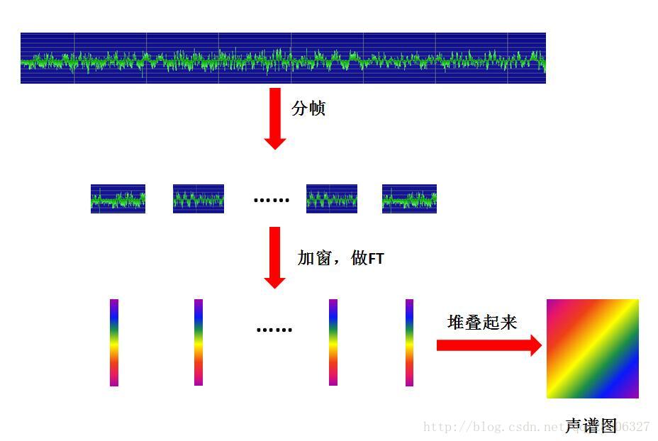
声音信号本是一维的时域信号，直观上很难看出频率变化规律。如果通过傅里叶变换把它变到频域上，虽然可以看出信号的频率分布，但是丢失了时域信息，无法看出频率分布随时间的变化。为了解决这个问题，很多时频分析手段应运而生。短时傅里叶，小波，Wigner分布等都是常用的时频域分析方法。

短时傅里叶变换（STFT）是最经典的时频域分析方法。傅里叶变换（FT）想必大家都不陌生，这里不做专门介绍。所谓短时傅里叶变换，顾名思义，是对短时的信号做傅里叶变化。那么短时的信号怎么得到的? 是长时的信号分帧得来的。这么一想，STFT的原理非常简单，把一段长信号分帧、加窗，再对每一帧做傅里叶变换（FFT），最后把每一帧的结果沿另一个维度堆叠起来，得到类似于一幅图的二维信号形式。如果我们原始信号是声音信号，那么通过STFT展开得到的二维信号就是所谓的声谱图：

梅尔频谱

声谱图往往是很大的一张图，为了得到合适大小的声音特征，往往把它通过梅尔标度滤波器组（mel-scale filter banks），变换为梅尔频谱。什么是梅尔滤波器组呢？这里要从梅尔标度（mel scale）说起。

梅尔标度，the mel scale，由Stevens，Volkmann和Newman在1937年命名。我们知道，频率的单位是赫兹（Hz），人耳能听到的频率范围是20-20000Hz，但人耳对Hz这种标度单位并不是线性感知关系。例如如果我们适应了1000Hz的音调，如果把音调频率提高到2000Hz，我们的耳朵只能觉察到频率提高了一点点，根本察觉不到频率提高了一倍。如果将普通的频率标度转化为梅尔频率标度，映射关系如下式所示：

å¾ä¸

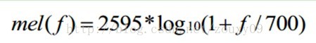
则人耳对频率的感知度就成了线性关系。也就是说，在梅尔标度下，如果两段语音的梅尔频率相差两倍，则人耳可以感知到的音调大概也相差两倍。
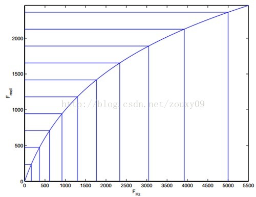
让我们观察一下从Hz到mel的映射图，由于它们是log的关系，当频率较小时，mel随Hz变化较快；当频率很大时，mel的上升很缓慢，曲线的斜率很小。这说明了人耳对低频音调的感知较灵敏，在高频时人耳是很迟钝的。

下面我们看代码：

fake_data_ph, _ = g_fn((noises_ph, one_hot_labels_ph))
fake_waves_ph = data_helper.data_to_waves(fake_data_ph)

这里g_fn索引进去就是生成器，noises_ph的shape是（8，256），8是batch_size，256还是latent vector size。one_hot_label_ph的shape是（8，61），8是batch_size，这里的61注意一下，因为MIDI的pitch范围是24~84，一共61个，所以是把这61个pitches映射成了one_hot label。然后输出的fake_data_ph的shape是（8，128，1024，2）。然后经过了data_to_wave函数（重点就在这一步，是怎么把最后G生成的东西转换为wave的，这个后面我们详细看一下data_to_wave函数，用到了上面提到的mel谱的知识），最后得到的fake_waves_ph的shape是（8，64000，1）。上面得到fake_data_ph这一步就用到了我们progressive Gan中的生成部分Generator，采用的是卷积神经网络（CNN），下面我们看一下Generator的模型结构。（论文中的表3）

这里我们可以了解到，G的输入是将Z和one_hot vector concat(连接）起来，所以输入为（1，1，61+256），也就是（1，1，317），G的输出的shape就是（128，1024，2），与fake_data_ph的shape相同。整个波形生成的过程是很复杂的，并不是Generator直接生成波形，而是一系列的信息的处理。

下面我们来追溯一下data_to_wave函数，这里用到的是mel谱，所以我们来看mel谱的data_to_wave:

class DataMelHelper(DataSTFTHelper):
  """A data helper for Mel Spectrograms."""

  def data_to_waves(self, data):
    return self.specgrams_helper.melspecgrams_to_waves(data)

这里输入的data就是刚才G生成的shape为（8，128，1024，2）的fake_data_ph，最后返回的是shape为(8,64000,1)的tensor。

下面我们接着来追溯这个self.specgrams_helper.melspecgrams_to_waves函数：

  def melspecgrams_to_waves(self, melspecgrams):

    """Converts mel-spectrograms to stfts."""
    return self.stfts_to_waves(self.melspecgrams_to_stfts(melspecgrams))

这么看来就是mel谱到wave其实是mel谱先转换为stft（短时傅里叶变换），然后再从stft转换为wave。我们看一下shape:

输入 melspecgrams的shape是(8,128,1024,2) ，self.melspecgrams_to_stfts(melspecgrams)的shape是(8,128,1024,1)，self.stfts_to_waves(self.melspecgrams_to_stfts(melspecgrams))的shape是(8,64000,1).

此时可以得出，mel谱转换为stft是把shape从(8,128,1024,2)——————>(8,128,1024,1)

stft转换为wave是把shape从(8,128,1024,1)——————>(8,64000,1)

下面我们先看mel谱转换为stft：

def melspecgrams_to_stfts(self, melspecgrams):
    """Converts mel-spectrograms to stfts."""
    return self.specgrams_to_stfts(self.melspecgrams_to_specgrams(melspecgrams))

这里可以看出从mel谱到stft其实是先将mel谱转化为声谱图，再将声谱图转换为stft。我们老样子，看一下shape:

输入 melspecgrams的shape是(8,128,1024,2) ，self.melspecgrams_to_specgrams(melspecgrams)输出的shape是(8,128,1024,2),self.specgrams_to_stfts(self.melspecgrams_to_specgrams(melspecgrams))的shape是(8,128,1024,1)。

此时可以得到，mel谱转换为声谱图是把shape从(8,128,1024,2)————>(8,128,1024,2)，shape不变

声谱图转换为stft是把shape从(8,128,1024,2)—————>(8,128,1024,1)，shape变了

下面：

specgrams: tensor of log magnitudes and instantaneous frequencies, shape[batch,time,freq,2];

melspecgrams: tensor of log magnitudes and instantaneous frequencies, shape[batch,time,freq,2];

stfts: complex64 tensor of stft,shape[batch,time,freq,1];

waves: tensor of waveform, shape[batch,time,1]。

从G的输出到wave简单画一下就是这样：

mel谱————>声谱图————>stft————>wave

shape变化是这样： (8,128,1024,2)————>(8,128,1024,2)————>(8,128,1024,1)————>(8,64000,1)

那么，可想而知，D正好反过来.

那么Generator的输入输出分别是什么呢？

答：从表3我们可以看出， G的输入是concat(Z,pitch),其中Z是就是latent vector，维度为256，pitch是维度为61的one-hot vector，将它们两个concat起来作为G的输入，维度就是（1，1，317）。经过一系列卷积和采样，最后输出的是size位（128，1024，2）的tensor,这个tensor是啥呢？我们来看看代码：

def generator_fn_specgram(inputs, **kwargs):
  """Builds generator network."""
  # inputs = (noises, one_hot_labels)
  with tf.variable_scope('generator_cond'):
    z = tf.concat(inputs, axis=1)
  if kwargs['to_rgb_activation'] == 'tanh':
    to_rgb_activation = tf.tanh
  elif kwargs['to_rgb_activation'] == 'linear':
    to_rgb_activation = lambda x: x
  fake_images, end_points = networks.generator(
      z,
      kwargs['progress'],
      lambda block_id: _num_filters_fn(block_id, **kwargs),
      kwargs['resolution_schedule'],
      num_blocks=kwargs['num_blocks'],
      kernel_size=kwargs['kernel_size'],
      colors=2,
      to_rgb_activation=to_rgb_activation,
      simple_arch=kwargs['simple_arch'])
  shape = fake_images.shape
  normalizer = data_normalizer.registry[kwargs['data_normalizer']](kwargs)
  fake_images = normalizer.denormalize_op(fake_images)
  fake_images.set_shape(shape)
  return fake_images, end_points

#其中networks.generator函数如下：
def generator(z,
              progress,
              num_filters_fn,
              resolution_schedule,
              num_blocks=None,
              kernel_size=3,
              colors=3,
              to_rgb_activation=None,
              simple_arch=False,
              scope='progressive_gan_generator',
              reuse=None):
  """Generator network for the progressive GAN model.

  Args:
    z: A `Tensor` of latent vector. The first dimension must be batch size.
    progress: A scalar float `Tensor` of training progress.
    num_filters_fn: A function that maps `block_id` to # of filters for the
        block.
    resolution_schedule: An object of `ResolutionSchedule`.
    num_blocks: An integer of number of blocks. None means maximum number of
        blocks, i.e. `resolution.schedule.num_resolutions`. Defaults to None.
    kernel_size: An integer of convolution kernel size.
    colors: Number of output color channels. Defaults to 3.
    to_rgb_activation: Activation function applied when output rgb.
    simple_arch: Architecture variants for lower memory usage and faster speed
    scope: A string or variable scope.
    reuse: Whether to reuse `scope`. Defaults to None which means to inherit
        the reuse option of the parent scope.
  Returns:
    A `Tensor` of model output and a dictionary of model end points.
  """
  if num_blocks is None:
    num_blocks = resolution_schedule.num_resolutions

  start_h, start_w = resolution_schedule.start_resolutions
  final_h, final_w = resolution_schedule.final_resolutions

  def _conv2d(scope, x, kernel_size, filters, padding='SAME'):
    return layers.custom_conv2d(
        x=x,
        filters=filters,
        kernel_size=kernel_size,
        padding=padding,
        activation=lambda x: layers.pixel_norm(tf.nn.leaky_relu(x)),
        he_initializer_slope=0.0,
        scope=scope)

  def _to_rgb(x):
    return layers.custom_conv2d(
        x=x,
        filters=colors,
        kernel_size=1,
        padding='SAME',
        activation=to_rgb_activation,
        scope='to_rgb')

  he_init = tf.contrib.layers.variance_scaling_initializer()

  end_points = {}

  with tf.variable_scope(scope, reuse=reuse):
    with tf.name_scope('input'):
      x = tf.contrib.layers.flatten(z)
      end_points['latent_vector'] = x

    with tf.variable_scope(block_name(1)):
      if simple_arch:
        x_shape = tf.shape(x)
        x = tf.layers.dense(x, start_h*start_w*num_filters_fn(1),
                            kernel_initializer=he_init)
        x = tf.nn.relu(x)
        x = tf.reshape(x, [x_shape[0], start_h, start_w, num_filters_fn(1)])
      else:
        x = tf.expand_dims(tf.expand_dims(x, 1), 1)
        x = layers.pixel_norm(x)
        # Pad the 1 x 1 image to 2 * (start_h - 1) x 2 * (start_w - 1)
        # with zeros for the next conv.
        x = tf.pad(x, [[0] * 2, [start_h - 1] * 2, [start_w - 1] * 2, [0] * 2])
        # The output is start_h x start_w x num_filters_fn(1).
        x = _conv2d('conv0', x, (start_h, start_w), num_filters_fn(1), 'VALID')
        x = _conv2d('conv1', x, kernel_size, num_filters_fn(1))
      lods = [x]

    if resolution_schedule.scale_mode == 'H':
      strides = (resolution_schedule.scale_base, 1)
    else:
      strides = (resolution_schedule.scale_base,
                 resolution_schedule.scale_base)

    for block_id in range(2, num_blocks + 1):
      with tf.variable_scope(block_name(block_id)):
        if simple_arch:
          x = tf.layers.conv2d_transpose(
              x,
              num_filters_fn(block_id),
              kernel_size=kernel_size,
              strides=strides,
              padding='SAME',
              kernel_initializer=he_init)
          x = tf.nn.relu(x)
        else:
          x = resolution_schedule.upscale(x, resolution_schedule.scale_base)
          x = _conv2d('conv0', x, kernel_size, num_filters_fn(block_id))
          x = _conv2d('conv1', x, kernel_size, num_filters_fn(block_id))
        lods.append(x)

    outputs = []
    for block_id in range(1, num_blocks + 1):
      with tf.variable_scope(block_name(block_id)):
        if simple_arch:
          lod = lods[block_id - 1]
          lod = tf.layers.conv2d(
              lod,
              colors,
              kernel_size=1,
              padding='SAME',
              name='to_rgb',
              kernel_initializer=he_init)
          lod = to_rgb_activation(lod)
        else:
          lod = _to_rgb(lods[block_id - 1])
        scale = resolution_schedule.scale_factor(block_id)
        lod = resolution_schedule.upscale(lod, scale)
        end_points['upscaled_rgb_{}'.format(block_id)] = lod

        # alpha_i is used to replace lod_select. Note sum(alpha_i) is
        # garanteed to be 1.
        alpha = _generator_alpha(block_id, progress)
        end_points['alpha_{}'.format(block_id)] = alpha

        outputs.append(lod * alpha)

    predictions = tf.add_n(outputs)
    batch_size = z.shape[0].value
    predictions.set_shape([batch_size, final_h, final_w, colors])
    end_points['predictions'] = predictions

  return predictions, end_points

这个卷积和采样过程中，变化的是频率分辨率？

具体过程是把patch变成one_hot labels，然后结合这61个latent vector生成假波形的相位，(label_ph, noise_ph) -> fake_wave_ph。

最后Combine audio from multiple notes into a single audio clip（那其实就是把这些notes连起来，但是有包络和normalize）。

[解析：这里的clip到底是指什么？我想是输入的噪声，通过MIDI文件中某些量的制定，通过padding，noemalize，相位，把所有notes连起来的wave。是频率与相位的完美结合。（猜想而已）]

最后这里涉及到一个知识点就是：振幅包络线（在振幅的频谱中，将各条频谱线的顶点练起来的曲线，称为振幅包络线）。

振幅包络线包括四个部分：

attack:起冲 Decay:衰减 Sustain:延留 Release:消去简称为ADSR(or ASDR)

当通过合成器来创造一个新声音时，这个合成器常常可以控制ADSR包络的形状，当使用录制好的声音进行创作时，想象ADSR包络的形状也是非常有用的。组合包络形状比较类似的声音可以帮助声音更好的结合在一起。

=============================================================================================

看完以上部分总结：那其实说白了输入到G的就是噪声，当然，MIDI文件中的量也会对生成的音乐有影响（我试了一个例子，MIDI是个字典，里面具有三个key,分别是pitch,start_time,end_time，这三个量对后面生成的音乐有一定的控制，当然，这与没有MIDI文件随机生成的音乐是有差别的）。

==============================================================================================

芝士小奶盖

关注

6
点赞
踩
30

收藏

觉得还不错? 一键收藏
10
评论
GANSYNTH（基于对抗性神经网络的音频合成）

本文基于文章《Adversarial neural audio synthesis》读了论文，看了源代码，还是有很多地方对不上，不理解（因为代码部分还是比较难的,音频音乐部分也涉及到很多信号处理方面的知识）。理解的我就补充进来。这是谷歌团队的megenta项目，首先先了解对抗神经网络（Gan，网上一大堆，可以找个demo看一看跑一跑就懂），以及progressive Gan,progr...
复制链接

扫一扫

专栏目录