论文解读《Semi-supervised Pathological Image Segmentation via Cross Distillation of Multiple Attentions》

论文解读《Semi-supervised Pathological Image Segmentation via Cross Distillation of Multiple Attentions》

基于多关注点交叉蒸馏的半监督病理图像分割

论文出处：MICCAI2023
论文地址：论文地址
代码地址：代码地址

一、摘要：
（1） 病理图像的分割是准确诊断肿瘤的关键步骤。然而，获取这些图像的密集注释用于训练是劳动密集型和耗时的。为了解决这个问题，半监督学习(SSL)具有降低标注成本的潜力，但它受到大量未标记训练图像的挑战。
（2） 提出了一种新的 基于多重关注交叉蒸馏(CDMA)的半监督方法 。
（3） 首先，我们提出了一个 多注意三分支网络(MTNet) 。其次，在三个解码器分支之间引入 交叉解码器知识蒸馏 (Cross Decoder Knowledge Distillation, CDKD)。
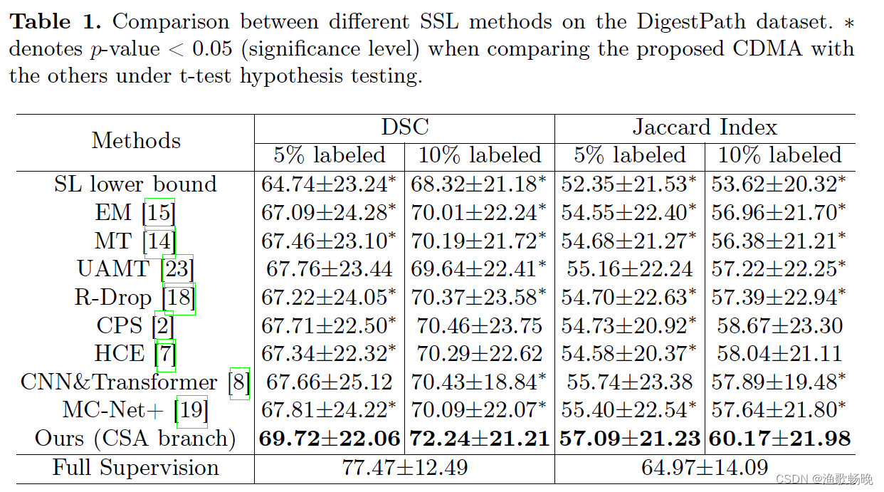
（4） 在DigestPath公共数据集上，将本文提出的CDMA与八种最先进的SSL方法进行了比较。

二、引言

（1） 在这项工作中，我们提出了一种新的 基于多关注交叉蒸馏(CDMA) 的半监督病理图像分割方法。
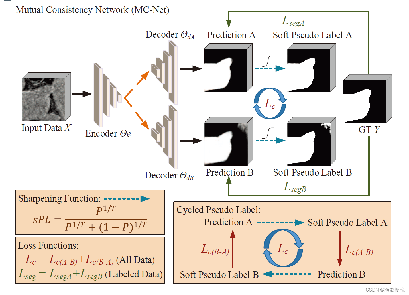
（2） 首先，提出了一种多注意力三分支网络(MTNet)。与MC-Net+[19]基于不同的上采样策略不同， 我们的MTNet在三个解码器分支中使用不同的注意机制 。
（3） 其次，受到最近研究中平滑标签对噪声鲁棒学习更有效的观察[10,22]的启发，我们 提出了一种交叉解码器知识蒸馏(CDKD)策略 。在CDKD中， 每个分支使用软标签监督作为其他两个分支的老师 。
（4） 此外，受EM[15]的启发，我们将 基于不确定性最小化的正则化应用于解码器之间的平均概率预测 。

二、方法

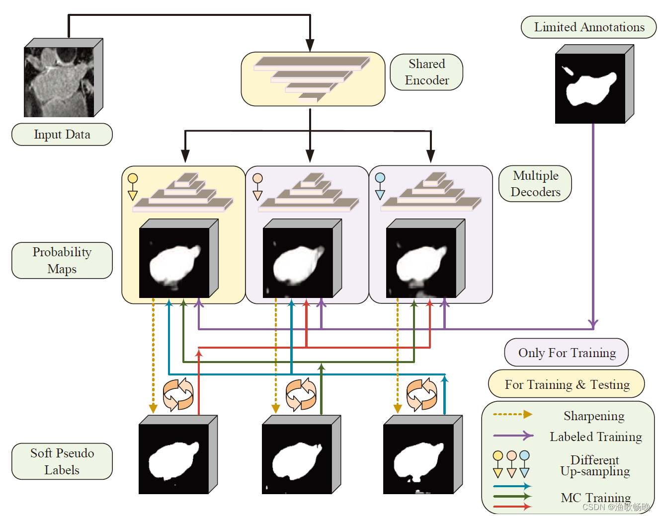
图1所示。我们的CDMA用于半监督分割。三个解码器分支使用不同的关注来获得不同的输出。为了更好地处理有噪声的伪标签，提出了交叉解码器知识蒸馏(CDKD)方法，并将不确定性最小化应用于三个分支的平均概率预测。Lsup仅用于标记图像。

2.1 多注意力三分支网络(MTNet)

(1) CA分支 通道注意块（channel attention blocks） :

其中F表示输入特征映射。和分别表示空间维度上的平均池化和最大池化。MLP和σ分别表示多层感知和sigmoid激活函数。Fc是由通道注意力校准的输出特征映射。

class ChannelAttention(nn.Module):
    def __init__(self, in_planes, ratio=16):
        super(ChannelAttention, self).__init__()
        self.avg_pool = nn.AdaptiveAvgPool2d(1)
        self.max_pool = nn.AdaptiveMaxPool2d(1)

        self.fc1 = nn.Conv2d(in_planes, in_planes // ratio, 1, bias=False)
        self.relu1 = nn.ReLU()
        self.fc2 = nn.Conv2d(in_planes // ratio, in_planes, 1, bias=False)
        self.sigmoid = nn.Sigmoid()

    def forward(self, x):
        avg_out = self.fc2(self.relu1(self.fc1(self.avg_pool(x))))
        max_out = self.fc2(self.relu1(self.fc1(self.max_pool(x))))
        out = avg_out + max_out
        return x*self.sigmoid(out)

(2) SA 分支 空间注意力 。SA块为:

其中Conv表示卷积层。和分别是通道维度上的平均池化和最大池化。⊕的意思是串联。

class SpatialAttention(nn.Module):
    def __init__(self, kernel_size=7):
        super(SpatialAttention, self).__init__()

        assert kernel_size in (3, 7), 'kernel size must be 3 or 7'
        padding = 3 if kernel_size == 7 else 1

        self.conv1 = nn.Conv2d(2, 1, kernel_size, padding=padding, bias=False)
        self.sigmoid = nn.Sigmoid()

    def forward(self, x):
        avg_out = torch.mean(x, dim=1, keepdim=True)
        max_out, _ = torch.max(x, dim=1, keepdim=True)
        y = torch.cat([avg_out, max_out], dim=1)
        y = self.conv1(y)
        return x*self.sigmoid(y)

(3) CSA 分支 对每个卷积块使用一个CSA块来校准特征映射。CSA块由CA块和SA块组成，同时利用信道和空间注意力。

class CBAM(nn.Module):
    def __init__(self, in_planes, ratio=16, kernel_size=7):
        super(CBAM, self).__init__()
        self.ca = ChannelAttention(in_planes, ratio)
        self.sa = SpatialAttention(kernel_size)
        
    def forward(self, x):
        out = self.ca(x)
        result = self.sa(out)
        return result

2.2交叉解码器知识蒸馏(CDKD)
引入了CDKD来增强MTNet利用未标记图像的能力，并消除带有噪声的伪标签的负面影响。它迫使每个解码器都受到其他两个解码器的软预测的监督。遵循KD[5]的做法，使用温度校准的Softmax (T-Softmax)来软化概率图:

式中，zc表示像素c类的logit预测值，pc表示c类的软概率值。温度T是控制输出概率软度的参数。注意，T = 1对应的是一个标准的Softmax函数，T值越大，概率分布越软，熵越高。当T<1时，式3 为锐化函数。
令PcA、PsA和PcsA分别表示TSoftmax对三个分支的软概率图。

另外两个分支为该分支的老师指导学习，CSA分支的KD损失为:

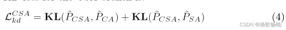
式中KL()为Kullback-Leibler散度函数。请注意，
的梯度只反向传播到CSA分支，因此知识是从教师提炼到学生的。同样，CA和SA分支的KD损失分别记为
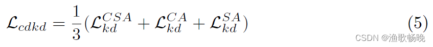
。则总蒸馏损失定义为:

class KDLoss(nn.Module):
    """
    Distilling the Knowledge in a Neural Network
    https://arxiv.org/pdf/1503.02531.pdf
    """

    def __init__(self, T):
        super(KDLoss, self).__init__()
        self.T = T

    def forward(self, out_s, out_t):
        loss = (
            F.kl_div(F.log_softmax(out_s / self.T, dim=1),
                     F.softmax(out_t / self.T, dim=1), reduction="batchmean") # , reduction="batchmean"
            * self.T
            * self.T
        )
        return loss
outputs1, outputs2, outputs3 = model(inputs)
kd_loss = KDLoss(T=10)
cross_loss1 = kd_loss(outputs1.permute(0, 2, 3, 1).reshape(-1, 2),outputs2.detach().permute(0, 2, 3, 1).reshape(-1, 2)) + \
            kd_loss(outputs1.permute(0, 2, 3, 1).reshape(-1, 2),outputs3.detach().permute(0, 2, 3, 1).reshape(-1, 2))
cross_loss2 = kd_loss(outputs2.permute(0, 2, 3, 1).reshape(-1, 2),outputs1.detach().permute(0, 2, 3, 1).reshape(-1, 2)) + \
    kd_loss(outputs2.permute(0, 2, 3, 1).reshape(-1, 2),outputs3.detach().permute(0, 2, 3, 1).reshape(-1, 2))
cross_loss3 = kd_loss(outputs3.permute(0, 2, 3, 1).reshape(-1, 2),outputs1.detach().permute(0, 2, 3, 1).reshape(-1, 2)) + \
    kd_loss(outputs3.permute(0, 2, 3, 1).reshape(-1, 2),outputs2.detach().permute(0, 2, 3, 1).reshape(-1, 2))
cross_consist = (cross_loss1 + cross_loss2 + cross_loss3)/3

KL散度（Kullback-Leibler Divergence，简称KL散度）是一种度量两个概率分布之间差异的指标，也被称为相对熵（Relative Entropy）。

2.3 基于平均预测的不确定性最小化
例如，两个分支分别预测像素的一种类别概率为0.0和1.0。为了避免这个问题，并进一步鼓励解码间的一致性，我们提出了一种基于平均预测的不确定性最小化方法:

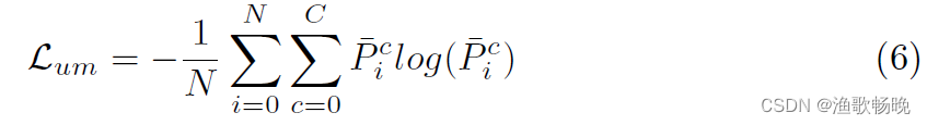
其中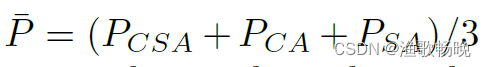
为平均概率图。C和N分别为类号和像素数量。P是像素i处c类的平均概率。

outputs1, outputs2, outputs3 = model(inputs)
outputs1_soft = torch.softmax(outputs1, dim=1)
outputs2_soft = torch.softmax(outputs2, dim=1)
outputs3_soft = torch.softmax(outputs3, dim=1)
outputs_avg_soft = (outputs1_soft+outputs2_soft+outputs3_soft)/3
en_loss = entropy_loss(outputs_avg_soft, C=2)

最后，我们的 CDMA的整体损失函数 为:

其中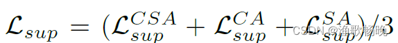
为标记训练图像上三个分支的平均监督学习损失，每个分支的监督学习损失计算概率预测(PcsA, PcA和PsA)与groundtruth标签之间的Dice损失和交叉熵损失。入1和入2分别是Lcdkd和Lum的权值。
都应用于标记和未标记的训练图像。

loss_sup = 0.5*dice_loss(outputs1_soft[:args.labeled_bs], labels[:args.labeled_bs])+0.5*F.cross_entropy(outputs1[:args.labeled_bs], labels[:args.labeled_bs,0,:,:].long()) + \
            0.5*dice_loss(outputs2_soft[:args.labeled_bs], labels[:args.labeled_bs])+0.5*F.cross_entropy(outputs2[:args.labeled_bs], labels[:args.labeled_bs,0,:,:].long()) + \
            0.5*dice_loss(outputs3_soft[:args.labeled_bs], labels[:args.labeled_bs])+0.5*F.cross_entropy(outputs3[:args.labeled_bs], labels[:args.labeled_bs,0,:,:].long())

        loss_sup = loss_sup/3

三、和其他方法对比

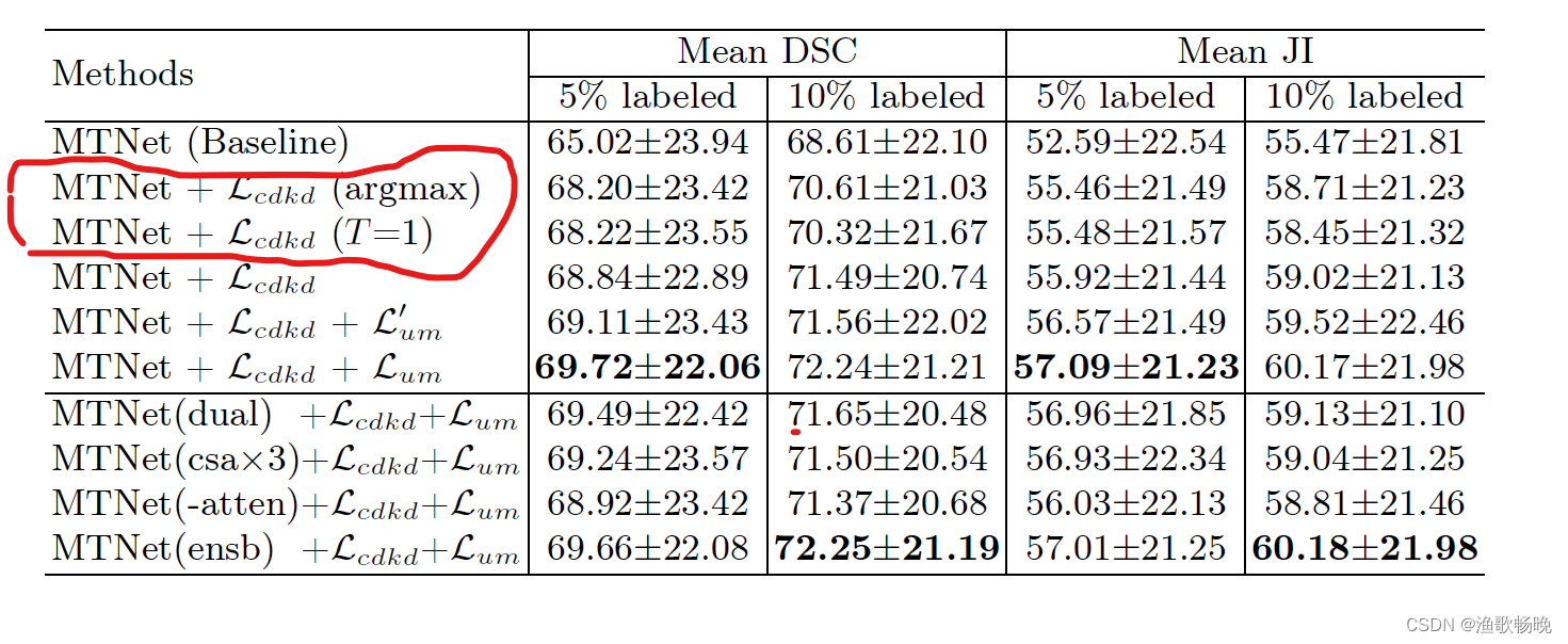
四、消融实验

五 结论

(1) 提出了一种基于多关注点交叉蒸馏(CDMA)的病理图像分割半监督框架。它采用多注意三分支网络，分别 基于渠道注意、空间注意和同时的渠道和空间注意生成多样化的预测 。
(2) 不同的基于注意的解码器分支关注特征映射的不同方面，导致不同的输出，这有利于半监督学习。为了消除训练中不正确的伪标签的负面影响
(3) 我们采用交叉解码器知识蒸馏(CDKD)来强制每个分支从其他两个分支生成的软标签中学习。
(4) 结肠镜组织分割数据集的实验结果表明，我们的CDMA优于八种最先进的SSL方法。在未来，将我们的方法应用于多类分割任务和来自不同器官的病理图像是有兴趣的。