一文读懂扩散模型，DDPM原理+代码解读

背景

图像生成领域最常见生成模型有GAN和VAE，2020年，DDPM（Denoising Diffusion Probabilistic Model）被提出，被称为扩散模型（Diffusion Model），同样可用于图像生成。近年扩散模型大热，OpenAI、Google Brain等相继基于扩散模型提出的以文生图，图像生成视频生成等模型。

原理介绍

扩散模型：和其他生成模型一样，实现从噪声（采样自标准正态分布）生成目标数据样本。
扩散模型包括两个过程：前向过程（forward process）和反向过程（reverse process），其中前向过程又称为扩散过程（diffusion process）。无论是前向过程还是反向过程都是一个参数化的马尔可夫链（Markov chain），其中反向过程可用于生成数据样本（它的作用类似GAN中的生成器，只不过GAN生成器会有维度变化，而DDPM的反向过程没有维度变化）。

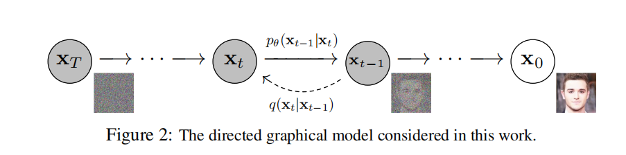
• $x_0$到$x_T$为逐步加噪过的前向程，噪声是已知的，该过程从原始图片逐步加噪至一组纯噪声。
• $x_T$到$x_0$为将一组随机噪声还原为输入的过程。该过程需要学习一个去噪过程，直到还原一张图片。

前向过程

前向过程是加噪的过程，前向过程中图像$x_t$只和上一时刻的$x_{t-1}$有关, 该过程可以视为马尔科夫过程, 满足:

• $q(x_{1:T}|x_0)={\prod }_{t=1}^{T}q(x_t|x_{t-1})$

• $q(x_t|x_{t-1})=N(x_t,\sqrt{1-{\beta }_t}{x}_{t-1},{\beta }_{t}I)$

其中不同t的${\beta }_t$是预先定义好的逐渐衰减的，可以是Linear，cosine等，满足${\beta }_1<{\beta }_2<...<{\beta }_T$。
${\beta }_t$生成代码如下：

def linear_beta_schedule(timesteps):
    scale = 1000 / timesteps
    beta_start = scale * 0.0001
    beta_end = scale * 0.02
    return np.linspace(beta_start, beta_end, timesteps).astype(np.float32)


def cosine_beta_schedule(time_steps, s=0.008):
    """
    cosine schedule
    as proposed in https://openreview.net/forum?id=-NEXDKk8gZ
    """
    steps = time_steps + 1
    x = np.linspace(0, time_steps, steps).astype(np.float32)
    alphas_cumprod = np.cos(((x / time_steps) + s) / (1 + s) * math.pi * 0.5) ** 2
    alphas_cumprod = alphas_cumprod / alphas_cumprod[0]
    betas = 1 - (alphas_cumprod[1:] / alphas_cumprod[:-1])
    return np.clip(betas, 0, 0.999)

根据以上公式，可以通过重参数化采样得到$x_t$。令$ϵ\sim N(0,I)$，${\alpha }_t=1-{\beta }_t$。${\overline{\alpha }}_t={\Pi }_{i=1}^T{\alpha }_i$
经过推导，可以得出$x_t$与$x_0$的关系：
$$q(x_t|x_0)=N(x_t;\sqrt{{\overline{\alpha }}_t}{x}_0,(1-{\overline{\alpha }}_t)I)$$

逆向过程

逆向过程是去噪的过程，如果得到逆向过程$q(x_{t-1}|x_t)$，就可以通过随机噪声$x_T$逐步还原出一张图像。DDPM使用神经网络$p_{\theta }(x_{t-1}|x_t)$拟合逆向过程$q(x_{t-1}|x_t)$。

$q(x_{t-1}|x_t,x_0)=N(x_{t-1}|\widetilde{{\mu }_t}(x_t,x_0),\widetilde{{\beta }_t}I)$，可以推导出:
$$p_{\theta }(x_{t-1}|x_t)=N(x_{t-1}|{\mu }_{\theta }(x_t,t),{\Sigma }_{\theta }(x_t,t))$$
DDPM论文中不计方差，通过神经网络拟合均值${\mu }_{\theta }$，从而得到$x_{t-1}$,

$${\mu }_{\theta }=\frac{1}{\sqrt{{\alpha }_t}}(x_t-\frac{1-{\alpha }_t}{\sqrt{1-\overline{{\alpha }_t}}}{ϵ}_{\theta (x_t,t)})$$

因为$t$和$x_t$已知，只需使用神经网络拟合${ϵ}_{\theta (x_t,t)}$

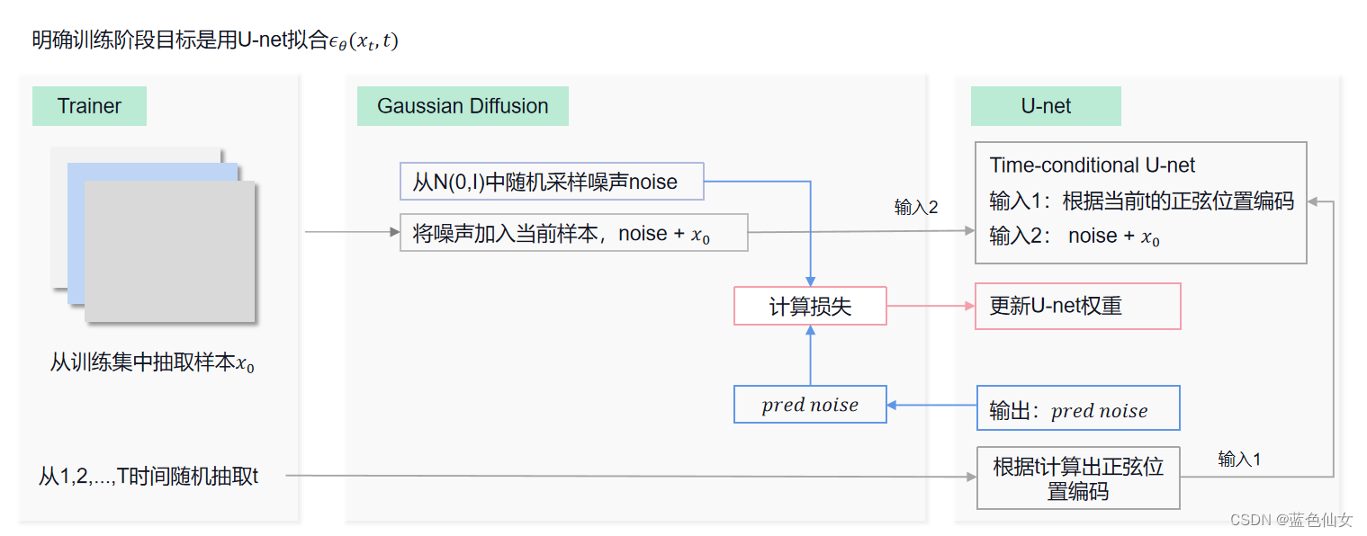
Unet职责

无论在前向过程还是反向过程，Unet的职责都是根据当前的样本和时间t预测噪声，也就是Unet实现${ϵ}_{\theta (x_t,t)}$的预测，整个训练过程其实就是在训练Unet网络的参数。

Gaussion Diffusion职责

前向过程：从1到T的时间采样一个时间t，生成一个随机噪声加到图片上，从Unet获取预测噪声，计算损失后更新Unet梯度
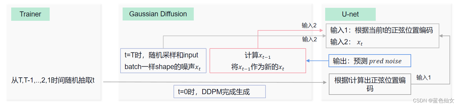
反向过程：先从正态分布随机采样和训练样本一样大小的纯噪声图片，从T-1到0逐步重复以下步骤：从xt还原xt-1。

训练过程

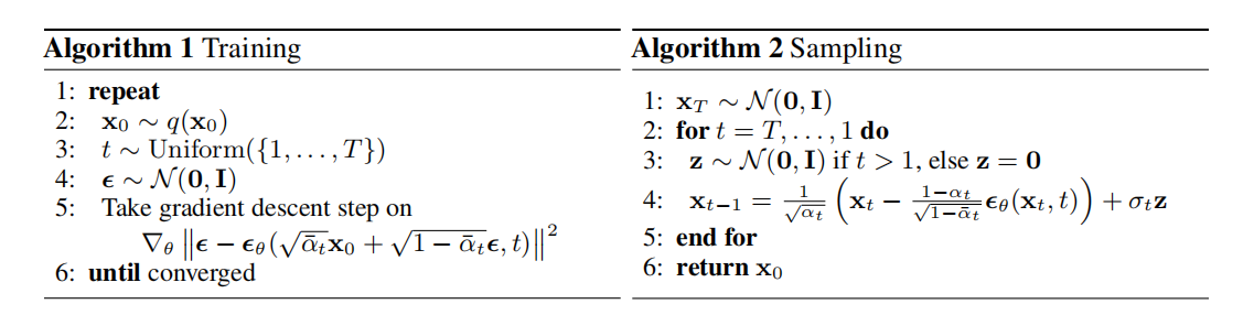
Algorithm1：Training：

• 从数据中抽取一个样本；
• 从1-T中随机选取一个时间t；
• 将$x_0$和t传给GaussionDiffusion，GaussionDiffusion采样一个随机噪声，加到$x_0$，形成$x_t$，然后将$x_t$和t放入Unet，Unet根据t生成正弦位置编码和$x_t$结合，Unet预测加的这个噪声，并返回噪声，GaussionDiffusion计算该噪声和随机噪声的损失；
• 将神经网络Unet预测的噪声与之前GaussionDiffusion采样的随机噪声求L2损失，计算梯度，更新权重；
• 重复以上步骤，直到网络Unet训练完成。

训练步骤中每个模块的交互如下图：

Algorithm2：Sampling

• 从标准正态分布采样出$x_T$；
• 从$T,T-1,...,2,1$依次重复以下步骤:
• （1）从标准正态分布采样$z$，为重参数化做准备；
• （2）根据模型求出${ϵ}_{\theta }$，计算出样本noise的均值，结合$x_t-prednoise$和$z$，利用重参数化技巧，得到$x_{t-1}$；
• 循环结束后返回$x_0$。

采样步骤中每个模块的交互如下图：

结合代码（MindSpore版本）讲解

代码主要分为以下几块：Unet、GaussianDiffusion、 Trainer

1. Unet相关模块

Unet网络结构如图：

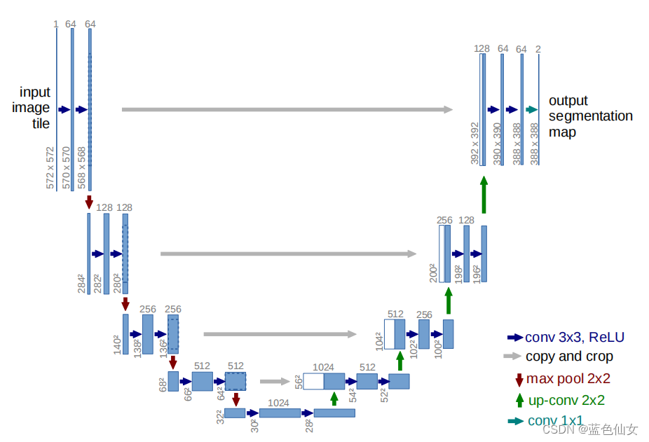
正弦位置编码

DDPM每步训练是随机采样一个时间，为了让网络知道当前处理的是一系列去噪过程中的哪一个step，我们需要将当前t编码并传入网络之中，DDPM使用的Unet是time-condition Unet。
类似于Transformer的positional embedding，DDPM采用正弦位置编码（Sinusoidal Positional Embeddings），既需要位置编码有界又需要两个时间步长之间的距离与句子长度无关。为了满足这两点标准，一种思路是使用有界的周期性函数，而简单的有界周期性函数很容易想到sin和cos函数。

class SinusoidalPosEmb(nn.Cell):
    def __init__(self, dim):
        super().__init__()
        half_dim = dim // 2
        emb = math.log(10000) / (half_dim - 1)
        emb = np.exp(np.arange(half_dim) * - emb)
        self.emb = Tensor(emb, mindspore.float32)
        self.Concat = _get_cache_prim(ops.Concat)(-1)

    def construct(self, x):
        emb = x[:, None] * self.emb[None, :]
        emb = self.Concat((ops.sin(emb), ops.cos(emb)))
        return emb

DDPM的Unet有ResidualBlock和Attention Module

Attention

Attention的本质是从人类视觉注意力机制中获得灵感(可以说很‘以人为本’了)。大致是我们视觉在感知东西的时候，一般不会是一个场景从到头看到尾每次全部都看，而往往是根据需求观察注意特定的一部分。具体可以参考博客：https://zhuanlan.zhihu.com/p/35571412

class Attention(nn.Cell):
    def __init__(self, dim, heads=4, dim_head=32):
        super().__init__()
        self.scale = dim_head ** -0.5
        self.heads = heads
        hidden_dim = dim_head * heads

        self.to_qkv = _get_cache_prim(Conv2d)(dim, hidden_dim * 3, 1, pad_mode='valid', has_bias=False)
        self.to_out = _get_cache_prim(Conv2d)(hidden_dim, dim, 1, pad_mode='valid', has_bias=True)
        self.map = ops.Map()
        self.partial = ops.Partial()
        self.bmm = BMM()
        self.split = ops.Split(axis=1, output_num=3)
        self.softmax = ops.Softmax(-1)

    def construct(self, x):
        b, c, h, w = x.shape
        qkv = self.split(self.to_qkv(x))
        q, k, v = self.map(self.partial(rearrange, self.heads), qkv)
        q = q * self.scale
        sim = self.bmm(q.swapaxes(2, 3), k)
        attn = self.softmax(sim)
        out = self.bmm(attn, v.swapaxes(2, 3))
        out = out.swapaxes(-1, -2).reshape((b, -1, h, w))
        return self.to_out(out)

Residual Block是ResNet的核心模块，可以防止网络退化。

class Residual(nn.Cell):
    """残差块"""
    def __init__(self, fn):
        super().__init__()
        self.fn = fn

    def construct(self, x, *args, **kwargs):
        return self.fn(x, *args, **kwargs) + x

2. GaussianDiffusion

首先定义相关的概率值，与公式相对应：

        self.betas = betas
        self.alphas_cumprod = alphas_cumprod
        self.alphas_cumprod_prev = alphas_cumprod_prev

        # calculations for diffusion q(x_t | x_{t-1}) and others
        self.sqrt_alphas_cumprod = Tensor(np.sqrt(alphas_cumprod))
        self.sqrt_one_minus_alphas_cumprod = Tensor(np.sqrt(1. - alphas_cumprod))
        self.log_one_minus_alphas_cumprod = Tensor(np.log(1. - alphas_cumprod))
        self.sqrt_recip_alphas_cumprod = Tensor(np.sqrt(1. / alphas_cumprod))
        self.sqrt_recipm1_alphas_cumprod = Tensor(np.sqrt(1. / alphas_cumprod - 1))

        posterior_variance = betas * (1. - alphas_cumprod_prev) / (1. - alphas_cumprod)

        self.posterior_variance = Tensor(posterior_variance)

        self.posterior_log_variance_clipped = Tensor(
            np.log(np.clip(posterior_variance, 1e-20, None)))
        self.posterior_mean_coef1 = Tensor(
            betas * np.sqrt(alphas_cumprod_prev) / (1. - alphas_cumprod))
        self.posterior_mean_coef2 = Tensor(
            (1. - alphas_cumprod_prev) * np.sqrt(alphas) / (1. - alphas_cumprod))

        p2_loss_weight = (p2_loss_weight_k + alphas_cumprod / (1 - alphas_cumprod))\
                          ** - p2_loss_weight_gamma
        self.p2_loss_weight = Tensor(p2_loss_weight)

计算损失

基于Unet预测出noise，使用预测noise和真实noise计算损失：

	def p_losses(self, x_start, t, noise, random_cond):
	    # 生成的真实noise
	    x = self.q_sample(x_start=x_start, t=t, noise=noise)
	
	    # if doing self-conditioning, 50% of the time, predict x_start from current set of times
	    if self.self_condition:
	        if random_cond:
	            _, x_self_cond = self.model_predictions(x, t)
	            x_self_cond = ops.stop_gradient(x_self_cond)
	        else:
	            x_self_cond = ops.zeros_like(x)
	    else:
	        x_self_cond = ops.zeros_like(x)
	
	    # model_out为基于Unet预测的pred_noise，此处self.model为Unet，ddpm默认预测目标是pred_noise。
	    model_out = self.model(x, t, x_self_cond)
	
	    if self.objective == 'pred_noise':
	        target = noise
	    elif self.objective == 'pred_x0':
	        target = x_start
	    elif self.objective == 'pred_v':
	        v = self.predict_v(x_start, t, noise)
	        target = v
	    else:
	        target = noise
		
		# 计算损失值
	    loss = self.loss_fn(model_out, target)
	    loss = loss.reshape(loss.shape[0], -1)
	    loss = loss * extract(self.p2_loss_weight, t, loss.shape)
	    return loss.mean()

采样

输出x_start，也就是原始图像，当sampling_time_steps< time_steps，用下方函数：

def ddim_sample(self, shape, clip_denoise=True):
    batch = shape[0]
    total_timesteps, sampling_timesteps, = self.num_timesteps, self.sampling_timesteps
    eta, objective = self.ddim_sampling_eta, self.objective

    # [-1, 0, 1, 2, ..., T-1] when sampling_timesteps == total_timesteps
    times = np.linspace(-1, total_timesteps - 1, sampling_timesteps + 1).astype(np.int32)
    # [(T-1, T-2), (T-2, T-3), ..., (1, 0), (0, -1)]
    times = list(reversed(times.tolist()))
    time_pairs = list(zip(times[:-1], times[1:]))

	# 采样第一次迭代，Unet输入img为随机采样
    img = np.random.randn(*shape).astype(np.float32)
    
    x_start = None

    for time, time_next in tqdm(time_pairs, desc='sampling loop time step'):
        # time_cond = ops.fill(mindspore.int32, (batch,), time)
        time_cond = np.full((batch,), time).astype(np.int32)
        x_start = Tensor(x_start) if x_start is not None else x_start
        self_cond = x_start if self.self_condition else None
        predict_noise, x_start, *_ = self.model_predictions(Tensor(img, mindspore.float32),
                                                            Tensor(time_cond),
                                                            self_cond,
                                                            clip_denoise)
        predict_noise, x_start = predict_noise.asnumpy(), x_start.asnumpy()
        if time_next < 0:
            img = x_start
            continue

        alpha = self.alphas_cumprod[time]
        alpha_next = self.alphas_cumprod[time_next]

        sigma = eta * np.sqrt(((1 - alpha / alpha_next) * (1 - alpha_next) / (1 - alpha)))
        c = np.sqrt(1 - alpha_next - sigma ** 2)

        noise = np.random.randn(*img.shape)

        img = x_start * np.sqrt(alpha_next) + c * predict_noise + sigma * noise

    img = self.unnormalize(img)

    return img

3. Trainer 训练器

data_iterator中每次取出的数据集就是一个batch_size大小，每训练一个batch，self.step就会加1。

指数移动平均

DDPM的trainer采用ema（指数移动平均）优化，ema不参与训练，只参与推理，比对变量直接赋值而言，移动平均得到的值在图像上更加平缓光滑，抖动性更小。具体代码参考代码仓中ema.py。

参数解读

• num_timesteps：原理中提到的T，扩散的步数
• train_num_steps：训练的总步数，每个step取用一个batch的数据。

print('training start')
        with tqdm(initial=self.step, total=self.train_num_steps, disable=False) as pbar:
            total_loss = 0.
            for (img,) in data_iterator:
                model.set_train()
                # 随机采样time向量
                time_emb = Tensor(
                    np.random.randint(0, num_timesteps, (img.shape[0],)).astype(np.int32))
                noise = Tensor(np.random.randn(*img.shape), mindspore.float32)
                # 返回损失、计算梯度、更新梯度
                self_cond = random.random() < 0.5 if self.self_condition else False
                loss = train_step(img, time_emb, noise, self_cond)

                # 损失累加
                total_loss += float(loss.asnumpy())

                self.step += 1
                if self.step % gradient_accumulate_every == 0:
                    # ema和model的参数同步更新
                    self.ema.update()
                    pbar.set_description(f'loss: {total_loss:.4f}')
                    pbar.update(1)
                    total_loss = 0.

                accumulate_step = self.step // gradient_accumulate_every
                accumulate_remain_step = self.step % gradient_accumulate_every
                if self.step != 0 and accumulate_step % self.save_and_sample_every == 0\
                        and accumulate_remain_step == 0:

                    self.ema.set_train(False)
                    self.ema.synchronize()
                    batches = num_to_groups(self.num_samples, self.batch_size)
                    all_images_list = list(map(lambda n: self.ema.online_model.sample(batch_size=n),
                                               batches))
                    self.save_images(all_images_list, accumulate_step)
                    self.save(accumulate_step)
                    self.ema.desynchronize()

                if self.step >= gradient_accumulate_every * self.train_num_steps:
                    break

        print('training complete')

相关论文

• Denoising Diffusion Probabilistic Models

代码链接

昇思大模型平台：https://xihe.mindspore.cn/projects/drizzlezyk/DDPM
启智：https://openi.pcl.ac.cn/drizzlezyk/ddpm2
Github：https://github.com/drizzlezyk/DDPM-MindSpore