CNN in Matlab

最新推荐文章于 2023-06-14 18:51:46 发布

岚大大

最新推荐文章于 2023-06-14 18:51:46 发布

阅读量1.1k

点赞数 2

分类专栏：图像处理机器学习编程小能手文章标签： MatConvNet

机器学习同时被 3 个专栏收录

5 篇文章 0 订阅

订阅专栏

图像处理

4 篇文章 0 订阅

订阅专栏

编程小能手

3 篇文章 0 订阅

订阅专栏

1.前言

最近需要用到卷积神经网络(CNN)，在还没完全掌握cuda+caffe+TensorFlow+python这一套传统的深度学习的流程的时候，想到了matlab，自己查了一下documentation,还真的有深度学习的相关函数。所以给自己提个醒，在需要用到某个成熟的技术时先查一下matlab的帮助文档，这样会减少很多时间成本。记得机器学习的大牛Andrew NG.说过在硅谷好多人都是先用matlab/octava先实现自己的想法，再转化成其他语言。

2.配置需求

要像用matlab实现deep learning，需要更新到2017a版本。GPU加速的话，需要安装cuda8.0, 自己GPU 的compute capacity 要3.0 以上。

3. 可以完成的任务

我们看一下matlab的新加的深度学习功能可以完成哪些任务

1. 获取别人训练好的CNN网络
2. 迁移学习(transfer learning and fine-tune)
3. 解决分类问题(classifiy problem)
4. 解决回归问题(regression problem)
5. 物体检测(object detection)
6. 提取学习到的特征

3.1 获取别人训练好的网络

matlab2017中，可以用别人训练好的现成的网络，也可以输入caffe中的网络。目前已知的可以用的网络包括用于分类的：Alexnet, vgg16, vgg19。已经用于物体检测的，RCNN, FastRCNN, Faster RCNN。由于最近一直研究的是分类和回归问题，物体检测的CNN在过后补全。这里只举一个分类的例子。
Alexnet作为2012年ImageNet的冠军，它的提出确实影响到了CV的研究热点，人们惊奇的发现深度网络的描述能力居然这么强，虽然背后的数学原理一直没能得到完美的解决，但不妨碍它强大的能力，我们看看她在matlab中是如何做分类的。首先贴出代码：

clear;clc;close all;
%获取alexnet
net = alexnet;  
%读照片选物体
I= imread('peppers.png'); 
[cropedim, rect2]=imcrop(I);
cropedim=imresize(cropedim,[227 227]);
figure,imshow(cropedim);
% 用AlexNet分类 
label = classify(net, cropedim); 
% 显示结果
figure; 
imshow(I); 
rectangle('position',rect2,'EdgeColor','r','LineWidth',2);
text(10,20,char(label),'Color','white','FontSize',20);

用matlab自带的照片测试一下分类的准确率，得到的结果如下

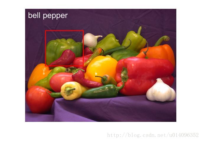
bell pepper是甜椒的意思，我们发现效果还是不错的，感兴趣的同学可以多找几张测试图片试一下。用

net.Layers

命令可以看Alnexnet的网络结构，得到以下

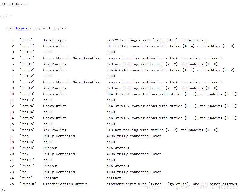
这是一个25层的网络，每一层都对应着详细的说明。值得关注的是有5个卷积层(convolution layer)和三个全连接层(full connection layer)。其他的vgg16和vgg19是相同的道理，不过要看清楚网络的输入，使用vgg19时，需要改变上边代码中的两行

net = vgg19;
cropedim=imresize(cropedim,[224 224]);

剩下的部分是一样的。当然也可以从caffe中导入自己训练好的网络，自己还没有完全掌握caffe,熟悉这部分的同学可以自己实现一下。

3.2 迁移学习(transfer learning and fine-tune)

所谓迁移学习(transfer learning)就是微调(fine-tune)别人训练好的网络中的某些参数，使得它更适合自己的数据集。迁移学习使用的情况是:几百到几千个训练样本，想快速训练网络。网络的训练过程就是刚开始为各个参数赋予随机的值，采用数值的方法(一般是梯度下降法)求让cost function 达到最小值的各个参数的取值，这些参数主要产生于各个层之间连接时候的权值。Cost function是标定好的数据与通过网络计算出的数据的差的累加。Cost function越小说明网络的性能越好。我们看看matlab中是如何用现有的网络做迁移学习的，我们举一个手写体识别的例子，其中matlab自己提供了训练集和测试集。先贴出代码：

%% transfer learning
%读取训练集和测试集
digitDatasetPath = fullfile(matlabroot,'toolbox','nnet','nndemos', ...
    'nndatasets','DigitDataset');
digitData = imageDatastore(digitDatasetPath, ...
    'IncludeSubfolders',true,'LabelSource','foldernames');
[trainDigitData,testDigitData] = splitEachLabel(digitData,0.5,'randomize');
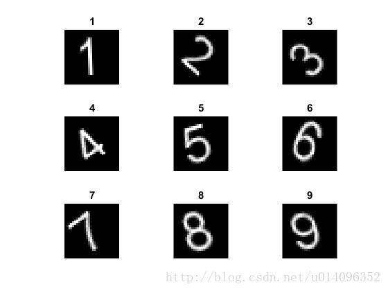
%显示前20个训练照片
numImages = numel(trainDigitData.Files);
idx = randperm(numImages,20);
for i = 1:20
    subplot(4,5,i)

    I = readimage(trainDigitData, idx(i));

    imshow(I)
end
% 获取matlab自己训练好的网络
load(fullfile(matlabroot,'examples','nnet','LettersClassificationNet.mat'))
% 改变输出层的类别个数
layersTransfer = net.Layers(1:end-3);
% 显示新的类别个数
numClasses =  numel(categories(trainDigitData.Labels));
% 把最后三层替换成新的类别
layers = [...
    layersTransfer
    fullyConnectedLayer(numClasses,'WeightLearnRateFactor',20,'BiasLearnRateFactor',20)
    softmaxLayer
    classificationLayer];
optionsTransfer = trainingOptions('sgdm',...
    'MaxEpochs',5,...
    'InitialLearnRate',0.0001,...
    'ExecutionEnvironment','cpu');
% 训练网络
netTransfer = trainNetwork(trainDigitData,layers,optionsTransfer);
% 显示测试准确率
YPred = classify(netTransfer,testDigitData);
YTest = testDigitData.Labels;
accuracy = sum(YPred==YTest)/numel(YTest);
% 显示测试结果
idx = 501:500:5000;
figure
for i = 1:numel(idx)
    subplot(3,3,i)

    I = readimage(testDigitData, idx(i));
    label = char(YTest(idx(i)));

    imshow(I)
    title(label)
end

代码的前边的部分是读取matlab中自带的数据集和测试集，把它保存成imageDatastore格式，这种格式只需要提供图片的路径信息而不用把图片全部读入内存中，因此非常适合大规模的数据集。中间部分是修改训练好的网络中的最后三层，原网络用来识别手写的字母和数字有36类，而现在的任务只需要识别手写体数字，所以把它们改成10类，在训练时使用0.0001的学习率，共计算5轮，用cpu做训练。代码的最后部分是测试新训练好的网络，因为transfer learn是在现有的网络基础上做参数的微调，所以训练速度很快，我们看一下训练效果。

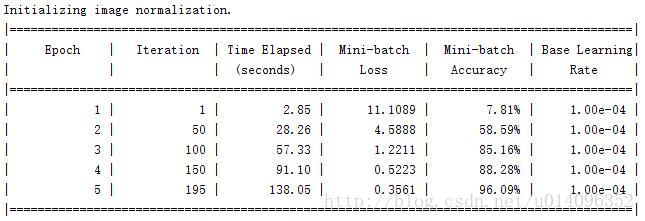
由于是在cpu上做的训练，而且是transfer learning 所以训练的过程很快，我们发现重新训练好的网络能达到很高的准确率。我们再看gpu上的训练
这里写图片描述

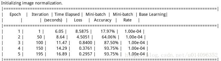
由于参数的初始化是随机的，因此得到的结果也是随机的，不过可以看出gpu上做训练明显要快很多！GPU的第一轮计算慢是因为数据要重新初始化为gpu矩阵。最后放一张效果图：
这里写图片描述

我们发现识别的效果还是不错的。

3.3 分类问题(classification problem)

CNN之所以能引起广泛关注，就是在于它最初在图像分类方面取得很大的成功，后来人们发现对于其他的分类问题，CNN也有很好的性能。上边讲的迁移学习解决的也是一种分类问题，接下来的叙述也就建立在上文的基础上。
我们这里要解决的分类问题，就是训练自己的分类网络。之前的迁移学习已经说明，所谓训练就是为每层网络之间寻找使得cost function最小的权值，这些权值刚开始是按照某种分布随机初始化的，我们用数值的方法求cost function的最小值。一般来说，我们用神经网络建立的是一个非常复杂的模型，我们往往能难找到这个模型的最小值，但可以找到它的极小值(局部最小值)，这些极小值已经很接近我们要找到最小值。
要训练自己的网络，我们要先建立自己的网络，并设置一定的训练参数。我们看一下matlabs是如何完成的。
在matlab中用来建立网络的语句如下：

layers = [ ...
    imageInputLayer([imsize imsize 1])
    convolution2dLayer(5,150)
    reluLayer
    crossChannelNormalizationLayer(5,'Alpha',0.00005,'Beta',0.75,'K',1)  %Norm layer1        
    convolution2dLayer(3,300,'Stride',1,'BiasLearnRateFactor',2)         %Cov2 layer
    reluLayer
    fullyConnectedLayer(1)
    softmaxLayer
    classificationLayer];

直接用数组建立网络，这个例子是建立一个9层的分类网络，包括输入层，卷积层1，激活函数层1，标准化层，卷积层2，激活函数层2，全连接层，去最大值层，分类层。至于如何选择适合自己的网络结构，我目前还没有搞太清楚，不过，可以现在别人的网络基础上做修改。
用来设定修改参数的语句如下：

options = trainingOptions('sgdm', ...
    'MaxEpochs',15, ...
    'InitialLearnRate',1e-4, ...
    'MiniBatchSize',256,...
    'ExecutionEnvironment','gpu');
    'OutputFcn',functions);

这些参数是CNN网络的基本参数，MaxEpoch是计算的轮数，它的值越大越容易收敛，InitialLearRate是学习率，太大模型可能不会收敛，太小则收敛的太慢。MiniBatchSize是每次处理的数据的个数，ExcutionEnviroment是训练网络的环境，可以在CPU(‘cpu’)上做，也可在GPU(‘gpu’)上做，可以并行(‘paralle’)，默认的情况是先测试gpu，如果不可用在测试gpu。在matlab上用gpu训练网络时需要cuda8.0, 显卡计算能力为3.0。这些参数可以用指令gpuDevice来查看。OutputFcn是可以在训练过程中调用的某些函数。比如：它可以用来画cost function值的变化。如何像可视化训练表格（上文输出的那些）某些数据可以调用相应的函数，我在回归问题时会再说明。
设定好网络结构和训练参数后，可以用

net = trainNetwork(trainData,layers,options);

来训练自己的网络，训练数据可以是ImageDatastore类型，可以是4-D数组，四个维度分别是长度，宽度，通道数，第几个图片。因为4-D数组是一次性装入到内存中的，如果数据量太大时慎用，小心内存不足。同样，我们举一个完整的例子，也是利用matlab自带的数据集去分类手写体。代码如下：

%读取数据集并保存成imageDatastore形式
digitDatasetPath = fullfile(matlabroot,'toolbox','nnet','nndemos',...
    'nndatasets','DigitDataset');
digitData = imageDatastore(digitDatasetPath,...
        'IncludeSubfolders',true,'LabelSource','foldernames');
%随机显示二十个训练集中的图片
figure;
perm = randperm(10000,20);
for i = 1:20
    subplot(4,5,i);
    imshow(digitData.Files{perm(i)});
end
%把数据集划分成训练集和测试集
trainingNumFiles = 750;
rng(1) % For reproducibility
[trainDigitData,testDigitData] = splitEachLabel(digitData,...
                trainingNumFiles,'randomize');
%建立自己的网络
layers = [imageInputLayer([28 28 1]);
          convolution2dLayer(5,20);
          reluLayer();
          maxPooling2dLayer(2,'Stride',2);
          fullyConnectedLayer(10);
          softmaxLayer();
          classificationLayer()];
%设定训练参数
options = trainingOptions('sgdm','MaxEpochs',20,...
    'InitialLearnRate',0.0001);
%训练网络
convnet = trainNetwork(trainDigitData,layers,options);
%测试网络
YTest = classify(convnet,testDigitData);
TTest = testDigitData.Labels;
accuracy = sum(YTest == TTest)/numel(TTest);
disp(accuracy);

我自己的训练结果如下：

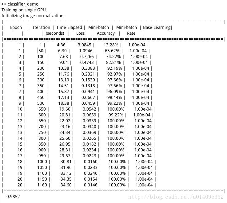
自己是在gpu上做的，所以时间较短，最后得到分类准确率发现还不错。

3.4 回归问题(regression problem)

回归问题与分类问题的处理方式相同，我们仍然需要训练集和测试集。在网路结构上有些不同，最后一次必须是Regression layer, 而倒数第二次必须是卷积层。回归问题的网络中的参数与分类问题是一样的，这里不再详细说明，我们直接分析一个例子，看一下matlab是如何做分类的。这个问题同时看一下function参数的作用。这次要解决的问题是，图片中的字母到底旋转了多少度。数据集同样来自matlab代码如下：

%读取数据集
[trainImages,~,trainAngles] = digitTrain4DArrayData;
%显示任意二十个结果
numTrainImages = size(trainImages,4);

figure
idx = randperm(numTrainImages,20);
for i = 1:numel(idx)
    subplot(4,5,i)

    imshow(trainImages(:,:,:,idx(i)))
    drawnow
end
%建立回归网络
layers = [ ...
    imageInputLayer([28 28 1])
    convolution2dLayer(12,25)
    reluLayer
    fullyConnectedLayer(1)
    regressionLayer];
%设置训练参数
functions={...
                @plotTrainingRMSE,...
                @(info)stopTrainingAtThreshold(info,0)};
options = trainingOptions('sgdm', ...
    'MaxEpochs',20, ...
    'InitialLearnRate',1e-3, ...
    'MiniBatchSize',128,...
    'ExecutionEnvironment','gpu',...
    'OutputFcn',functions);
%训练网络
net = trainNetwork(trainImages,trainAngles,layers,options);
%测试网络
[testImages,~,testAngles] = digitTest4DArrayData;
predictedTestAngles = predict(net,testImages);
%查看拟合误差
predictionError = testAngles - predictedTestAngles;
thr = 10;
numCorrect = sum(abs(predictionError) < thr);
numTestImages = size(testImages,4);
accuracy = numCorrect/numTestImages;
disp('accuracy');
disp(accuracy);
squares = predictionError.^2;
rmse = sqrt(mean(squares));
disp('the rmse');
disp(rmse);
%train function
function plotTrainingRMSE(info)

persistent plotObj

if info.State == "start"
    figure;
    plotObj = animatedline;
    xlabel("Iteration")
    ylabel("Training RMSE")
elseif info.State == "iteration"
    addpoints(plotObj,info.Iteration,double(info.TrainingRMSE))
    drawnow limitrate nocallbacks
end

end

function stop = stopTrainingAtThreshold(info,thr)

stop = false;
if info.State ~= "iteration"
    return
end

persistent TrainingRMSE

% Append accuracy for this iteration
T= info.TrainingRMSE;

% Evaluate mean of iteration accuracy and remove oldest entry

 stop = T <thr;

end

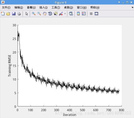
得到的回归结果如下：

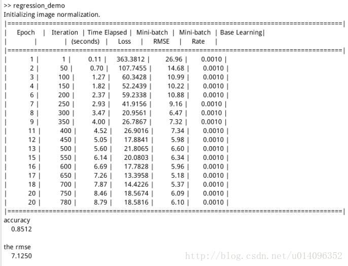
我们在训练过程中调用两个函数，plotTrainingRMSE是用来画cost function是如何变化的，(info)stopTrainingAtThreshold(info,0)是设置训练提前结束的条件的，可以根据表中的某些参数让训练在一定条件下停下来。最后，我们看一下cost function 的变换规律，如下：
这里写图片描述

目前为止，我们用cnn解决了最基本的分类问题和回归问题，此外，还介绍了如何建立网络和设定参数，后边将补充检测部分。

3.3 检测问题(Detection problem)

同样用matlab自带数据集做车辆检测，关于检测的网络有RCNN, Fast RCNN, Faster RCNN, 他们大同小异，差距在于速度的快慢，我们只测试Faster RCNN
1) 读取数据

data = load('fasterRCNNVehicleTrainingData.mat');

data是个结构体类型的数据，主要是用来四个属性分别是detector, layers, result, vehicleTraining.
其中，detector, layers, reault是提前训练好的检测子，网络和测试结果，我们用vehicleTraining重新训练CNN网络，用layers来设计网络结构
2) 抽取用于训练的图像

trainingData = data.vehicleTrainingData;
trainingData.imageFilename=fullfile(toolboxdir('vision'),'visiondata',...
trainingData.imageFilename);

抽取出的trainingData是table格式的，matlab训练网络RCNN网络只能用table格式。

3) 读取网络结构

layers=data.layers;

该网络是个11层的网络，训练时我们可以设计自己的网络结构，也可以在这个网络的基础上做训练。

4) 设置训练选项

options = trainingOptions('sgdm', ...
    'InitialLearnRate',1e-6,...
    'MaxEpochs',1,...
    'ExecutionEnvironment','gpu',...
    'CheckpointPath',tempdir);

这里设置的是初始学习率为 1e-6, 迭代1轮，用GPU做训练，在训练时会把checkpoint的结果存下来。

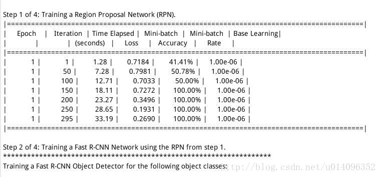
5) 训练网络

detector = trainFasterRCNNObjectDetector(trainingData,layers,options);

用trainingData做训练数据，训练layers网络，在训练过程中选择option中的训练参数，同样用了GPU做训练，其中的一步如下：

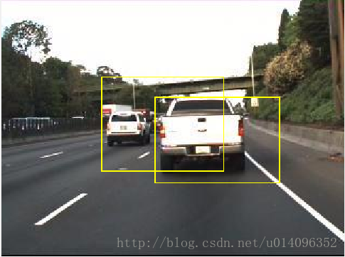
6) 结果检测

img=imread('highway.png');
[bbox,score,label]=detect(detector,img);
detectedImg=insertShape(img,'Rectangle',bbox);
figure,imshow(detectedImg);

从Matlab自身图库中选择hightway这张照片，用刚才训练出的网络监测里边的车辆，其中bbox是监测出的包围盒的坐标，这个可以用来返回。
这结果显示如下：

岚大大

关注

2
点赞
踩
11

收藏

觉得还不错? 一键收藏
0
评论
CNN in Matlab

1.前言最近需要用到卷积神经网络(CNN)，在还没完全掌握cuda+caffe+TensorFlow+python这一套传统的深度学习的流程的时候，想到了matlab，自己查了一下documentation,还真的有深度学习的相关函数。所以给自己提个醒，在需要用到某个成熟的技术时先查一下matlab的帮助文档，这样会减少很多时间成本。记得机器学习的大牛Andrew NG.说过在硅谷好多人都是先用m...
复制链接

扫一扫

专栏目录