Timothy Sauer版《数值分析》学习笔记+python实现——《常微分方程》（II）

Ordinary Differential Equation

Import package

import numpy as np
import matplotlib.pyplot as plt
from matplotlib.ticker import MaxNLocator
plt.rc("font", family="Times New Roman")
from tqdm import tqdm
import imageio
from mpl_toolkits.mplot3d import Axes3D

System of ODE

Pendulum

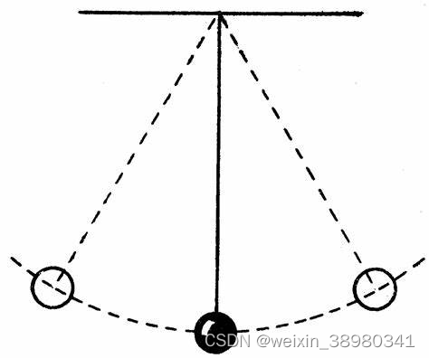
According to Newton’s Second Law:
$$\{\begin{array}{c}ml\ddot{x}+mgx=0\\ x\left(0\right)=\frac{\pi }{2}\\ \dot{x}\left(0\right)=0\end{array}$$
set: $x_1\left(t\right)=x,x_2\left(t\right)=\dot{x}$:
$$\{\begin{array}{c}{\dot{x}}_1=f\left(t,x_1\right)=x_2\\ x_1\left(0\right)=\frac{\pi }{2}\end{array};\{\begin{array}{c}{\dot{x}}_2=f\left(t,x_2\right)=-\frac{g}{l}{x}_1\\ x_2\left(0\right)=0\end{array}$$
When using the second-order Taylor method, note that:
$$\begin{gathered} f^{\prime }\left(t,x_1\right)=f_t+f_{x_1}f=f_t={\dot{x}}_2=-\frac{g}{l}{x}_1 \\ {f}^{\prime }\left(t,x_2\right)=f_t+f_{x_2}f=f_t=-\frac{g}{l}{\dot{x}}_1=-\frac{g}{l}{x}_2 \end{gathered}$$

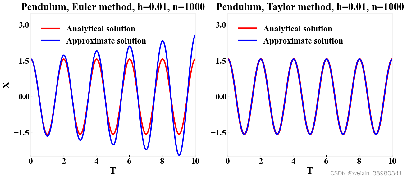
Next, apply the explicit Trapezoidal rule to solve the two ODEs.

g, l = 9.81, 1.0  # g = 9.81 m/s-2, l = 1 m
def real_func(t):  # analytical solution : x(t) = pi/2 * cos(wt), w = sqrt(g/l)
    return np.pi/2 * np.cos(np.sqrt(g/l) * t)

def SolveODE(y10, y20, step_h=0.01, n=1000):  # t from 0 -> 10
    omega1 = np.array([0] * (n + 1), dtype=float)  # x1 using Euler method
    omega2 = np.array([0] * (n + 1), dtype=float)  # x2 using Euler method
    omega3 = np.array([0] * (n + 1), dtype=float)  # x1 using 2-order Taylor method
    omega4 = np.array([0] * (n + 1), dtype=float)  # x2 using 2-order Taylor method
    omega1[0] = y10 
    omega2[0] = y20 
    omega3[0] = y10
    omega4[0] = y20
    for i in range(n):
        # Euler method:
        omega1[i + 1] = omega1[i] + step_h * omega2[i]  
        omega2[i + 1] = omega2[i] + step_h * (-g/l * omega1[i])
        # 2-order Taylor:
        omega3[i + 1] = omega3[i] + step_h * omega4[i] + np.power(step_h, 2)/2 * (-g/l * omega3[i])  
        omega4[i + 1] = omega4[i] + step_h * (-g/l * omega3[i]) + np.power(step_h, 2)/2 * (-g/l * omega4[i])
    return omega1, omega2, omega3, omega4 

t = np.linspace(0, 10, 1001)
x = real_func(t)
ret_euler, _, ret_taylor, _ = SolveODE(y10=np.pi/2, y20=0)

# plot:
plt.rcParams['xtick.direction'] = "in"  # ticks direction
plt.rcParams['ytick.direction'] = "in" 
plt.figure(figsize=(15, 6))
plt.subplot(1, 2, 1)
axes=plt.gca()
axes.yaxis.set_major_locator(MaxNLocator(5))  # ticks num
axes.xaxis.set_major_locator(MaxNLocator(5))
plt.axis([0, 10, -2.5, 3.5])  # ticks range (xinf, xsup, yinf, ysup)
plt.xticks(fontsize=20, fontweight="bold")  # ticks font
plt.yticks(fontsize=20, fontweight="bold")  
plt.xlabel("T", fontsize=22, fontweight="bold")
plt.ylabel("X", fontsize=22, fontweight="bold")
plt.title("Pendulum, Euler method, h=0.01, n=1000", fontsize=24, fontweight="bold")
plt.plot(t, x, color="red", linewidth=3, label="Analytical solution")
plt.plot(t, ret_euler, color="blue", linewidth=3, label="Approximate solution")
# set legend:
legend_font = {
    "family": "Times New Roman", 
    "style" : "normal",
    "size" : 20, 
    'weight': "bold"
}
plt.legend(
    bbox_to_anchor=(0.75, .72), loc="lower right", 
    frameon=False, prop=legend_font
)
plt.subplot(1, 2, 2)
axes=plt.gca()
axes.yaxis.set_major_locator(MaxNLocator(5))  # ticks num
axes.xaxis.set_major_locator(MaxNLocator(5))
plt.axis([0, 10, -2.5, 3.5])  # ticks range (xinf, xsup, yinf, ysup)
plt.xticks(fontsize=20, fontweight="bold")  # ticks font
plt.yticks(fontsize=20, fontweight="bold")  
plt.xlabel("T", fontsize=22, fontweight="bold")
plt.title("Pendulum, Taylor method, h=0.01, n=1000", fontsize=24, fontweight="bold")
plt.plot(t, x, color="red", linewidth=4, label="Analytical solution")
plt.plot(t, ret_taylor, color="blue", linewidth=3, label="Approximate solution")
# set legend:
legend_font = {
    "family": "Times New Roman", 
    "style" : "normal",
    "size" : 20, 
    'weight': "bold"
}
plt.legend(
    bbox_to_anchor=(0.75, .72), loc="lower right", 
    frameon=False, prop=legend_font
)
plt.show()

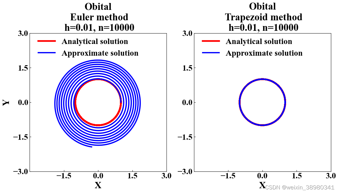
Orbital mechanics

Assuming that the star is at the origin, the Equations of motion of the planet located $(x,y)$ (only considering the $XOY$ plane) subject to universal gravitation is:
$$m_1\ddot{x}=-\frac{G{m}_1{m}_{2}x}{{\left(x^2+y^2\right)}^{3/2}}$$
$$m_1\ddot{y}=-\frac{G{m}_1{m}_{2}y}{{\left(x^2+y^2\right)}^{3/2}}$$
which can be transformed into four first order differential equations:
$$\dot{x}=v_x;x\left(0\right)=1$$
$${\dot{v}}_x=-\frac{G{m}_{2}x}{{\left(x^2+y^2\right)}^{3/2}};v_x\left(0\right)=0$$
$$\dot{y}=v_y;y\left(0\right)=0$$
$${\dot{v}}_y=-\frac{G{m}_{2}y}{{\left(x^2+y^2\right)}^{3/2}};v_y\left(0\right)=1$$

Gm = 1.0

def real_x(t):
    return np.cos(t)

def real_y(t):
    return np.sin(t)

def EulerSolveODE(x0, vx0, y0, vy0, step_h=0.01, n=10000):  # solve ODE by Euler method, t from 0 -> 100
    omega1 = np.array([0] * (n + 1), dtype=float)  # x
    omega2 = np.array([0] * (n + 1), dtype=float)  # vx
    omega3 = np.array([0] * (n + 1), dtype=float)  # y
    omega4 = np.array([0] * (n + 1), dtype=float)  # vy
    omega1[0] = x0 
    omega2[0] = vx0 
    omega3[0] = y0
    omega4[0] = vy0
    for i in range(n):
        omega1[i + 1] = omega1[i] + step_h * omega2[i]  
        omega2[i + 1] = omega2[i] + step_h * ((-Gm * omega1[i])/np.power((np.power(omega1[i], 2) + np.power(omega3[i], 2)), 3/2))
        omega3[i + 1] = omega3[i] + step_h * omega4[i]
        omega4[i + 1] = omega4[i] + step_h * ((-Gm * omega3[i])/np.power((np.power(omega1[i], 2) + np.power(omega3[i], 2)), 3/2))
    return omega1, omega2, omega3, omega4

def TrapezoidSolveODE(x0, vx0, y0, vy0, step_h=0.01, n=10000):  # solve ODE by Euler method, t from 0 -> 100
    omega1 = np.array([0] * (n + 1), dtype=float)  # x
    omega2 = np.array([0] * (n + 1), dtype=float)  # vx
    omega3 = np.array([0] * (n + 1), dtype=float)  # y
    omega4 = np.array([0] * (n + 1), dtype=float)  # vy
    omega1[0] = x0 
    omega2[0] = vx0 
    omega3[0] = y0
    omega4[0] = vy0
    for i in range(n):
        # pre-calculation using Euler method
        omega1[i + 1] = omega1[i] + step_h * omega2[i]  
        omega2[i + 1] = omega2[i] + step_h * ((-Gm * omega1[i])/np.power((np.power(omega1[i], 2) + np.power(omega3[i], 2)), 3/2))
        omega3[i + 1] = omega3[i] + step_h * omega4[i]
        omega4[i + 1] = omega4[i] + step_h * ((-Gm * omega3[i])/np.power((np.power(omega1[i], 2) + np.power(omega3[i], 2)), 3/2))
        # calculation using trapezoid method
        omega1[i + 1] = omega1[i] + step_h/2 * (omega2[i] + omega2[i + 1])
        omega2[i + 1] = omega2[i] + step_h/2 * ((-Gm * omega1[i])/np.power((np.power(omega1[i], 2) + np.power(omega3[i], 2)), 3/2) + (-Gm * omega1[i + 1])/np.power((np.power(omega1[i + 1], 2) + np.power(omega3[i + 1], 2)), 3/2))
        omega3[i + 1] = omega3[i] + step_h/2 * (omega4[i]+ omega4[i + 1])  
        omega4[i + 1] = omega4[i] + step_h/2 * ((-Gm * omega3[i])/np.power((np.power(omega1[i], 2) + np.power(omega3[i], 2)), 3/2) + (-Gm * omega3[i + 1])/np.power((np.power(omega1[i + 1], 2) + np.power(omega3[i + 1], 2)), 3/2))
    return omega1, omega2, omega3, omega4

t = np.linspace(0, 100, 10001)
r_x = real_x(t)
r_y = real_y(t)
euler_x, _, euler_y ,_ = EulerSolveODE(x0=1.0, vx0=0.0, y0=0.0, vy0=1.0)
trap_x, _, trap_y ,_ = TrapezoidSolveODE(x0=1.0, vx0=0.0, y0=0.0, vy0=1.0)

# plot:
plt.rcParams['xtick.direction'] = "in"  # ticks direction
plt.rcParams['ytick.direction'] = "in" 
plt.figure(figsize=(13, 6))
plt.subplot(1, 2, 1)
axes=plt.gca()
axes.yaxis.set_major_locator(MaxNLocator(5))  # ticks num
axes.xaxis.set_major_locator(MaxNLocator(5))
plt.axis([-3 + 0.0001, 3, -3, 3])  # ticks range (xinf, xsup, yinf, ysup)
plt.xticks(fontsize=20, fontweight="bold")  # ticks font
plt.yticks(fontsize=20, fontweight="bold")  
plt.xlabel("X", fontsize=22, fontweight="bold")
plt.ylabel("Y", fontsize=22, fontweight="bold")
plt.title("Obital\n Euler method\n h=0.01, n=10000", fontsize=24, fontweight="bold")
plt.plot(r_x, r_y, color="red", linewidth=4, label="Analytical solution")
plt.plot(euler_x, euler_y, color="blue", linewidth=3, label="Approximate solution")
# set legend:
legend_font = {
    "family": "Times New Roman", 
    "style" : "normal",
    "size" : 20, 
    'weight': "bold"
}
plt.legend(
    bbox_to_anchor=(0.85, .77), loc="lower right", 
    frameon=False, prop=legend_font
)
plt.subplot(1, 2, 2)
axes=plt.gca()
axes.yaxis.set_major_locator(MaxNLocator(5))  # ticks num
axes.xaxis.set_major_locator(MaxNLocator(5))
plt.axis([-3 + 0.0001, 3, -3, 3])  # ticks range (xinf, xsup, yinf, ysup)
plt.xticks(fontsize=20, fontweight="bold")  # ticks font
plt.yticks(fontsize=20, fontweight="bold")  
plt.xlabel("X", fontsize=22, fontweight="bold")
plt.title("Obital\n Trapezoid method\n h=0.01, n=10000", fontsize=24, fontweight="bold")
plt.plot(r_x, r_y, color="red", linewidth=4, label="Analytical solution")
plt.plot(trap_x, trap_y, color="blue", linewidth=3, label="Approximate solution")
# set legend:
legend_font = {
    "family": "Times New Roman", 
    "style" : "normal",
    "size" : 20, 
    'weight': "bold"
}
plt.legend(
    bbox_to_anchor=(0.85, .77), loc="lower right", 
    frameon=False, prop=legend_font
)
plt.show()

Three-body motion

$Velocity-VelertAlgorithm$:
$$x\left(t+\Delta t\right)=x\left(t\right)+v_x\left(t\right)\Delta t+\frac{1}{2}{a}_x\left(t\right){\left(\Delta t\right)}^2$$
$$v_x\left(t+\frac{\Delta t}{2}\right)=v_x\left(t\right)+\frac{1}{2}{a}_x\left(t\right)\Delta t$$
$$v_x\left(t+\Delta t\right)=v_x\left(t+\frac{\Delta t}{2}\right)+\frac{1}{2}{a}_x\left(t+\Delta t\right)\Delta t$$
$$a_{x,i}\left(t\right)=\sum _{i\ne j}\frac{G{m}_j}{R_{ij}^3}\left(x_j-x_i\right)$$
Reference: https://www.guanjihuan.com/archives/858

config = {
    "G" : 1.0,  # gravitational constant
    "N_steps" : 1e5,  # total step for motion
    "time_step" : 0.05,  # time step
    "observation_max" : 100,  # field of view when visualize the motion
    "out_frame" : 1000,  # save image per $out_frame$ steps
    "root" : "./three-body/"
}

class Ball:
    def __init__(self, m, x0=0, y0=0, vx0=0, vy0=0):
        self.mass = m  # mass
        self.x, self.y = np.array([x0], dtype=float), np.array([y0], dtype=float)  # initial position
        self.vx, self.vy = np.array([vx0], dtype=float), np.array([vy0], dtype=float)  # initial velocity
        self.ax, self.ay = 0.0, 0.0  # acceleration
    
    def distance(self, other, step):  # distance between two ball at this step
        return np.sqrt(np.power(self.x[step] - other.x[step], 2) + np.power(self.y[step] - other.y[step], 2))
    
    def CalculateAcceleration(self, others, step):  # acceleration at this step
        if type(others) == list:  # many body question
            self.ax, self.ay = 0.0, 0.0
            for other in others:
                if self.distance(other, step) != 0:
                    self.ax += config["G"] * other.mass * (other.x[step] - self.x[step])/np.power(self.distance(other, step), 3)
                    self.ay += config["G"] * other.mass * (other.y[step] - self.y[step])/np.power(self.distance(other, step), 3)
        else:  # monomer problem
            self.ax = config["G"] * other.mass * (other.x - self.x)/np.power(self.distance(other, step), 3)
            self.ay = config["G"] * other.mass * (other.y - self.y)/np.power(self.distance(other, step), 3)


def VelocityVerlert(ball_list, step, delta_t):
    for ball in ball_list:  # update coordinate
        ball.x[step + 1] = ball.x[step] + ball.vx[step] * delta_t + 0.5 * ball.ax * np.power(delta_t, 2)
        ball.y[step + 1] = ball.y[step] + ball.vy[step] * delta_t + 0.5 * ball.ay * np.power(delta_t, 2)
        ball.vx[step + 1] = ball.vx[step] + 0.5 * ball.ax * delta_t  # v(t + delta_t/2)
        ball.vy[step + 1] = ball.vy[step] + 0.5 * ball.ay * delta_t
    for ball in ball_list:  # updata velocity
        ball.CalculateAcceleration(ball_list, step + 1)
        ball.vx[step + 1] = ball.vx[step + 1] + 0.5 * ball.ax * delta_t  # real v(t + delta_t)
        ball.vy[step + 1] = ball.vy[step + 1] + 0.5 * ball.ay * delta_t

# set balls
ball1 = Ball(m=15, x0=300, y0=50, vx0=0, vy0=0)
ball2 = Ball(m=12, x0=-100, y0=-200, vx0=0, vy0=0)
ball3 = Ball(m=8, x0=-100, y0=150, vx0=0, vy0=0)
ball_list = [ball1, ball2, ball3]
# motion simulation
print("start simulation")
for ball in ball_list:  # initialization
    ball.x = np.append(ball.x, [0] * int(config["N_steps"] + 1 - len(ball.x)))
    ball.y = np.append(ball.y, [0] * int(config["N_steps"] + 1 - len(ball.y)))
    ball.vx = np.append(ball.vx, [0] * int(config["N_steps"] + 1 - len(ball.vx)))
    ball.vy = np.append(ball.vy, [0] * int(config["N_steps"] + 1 - len(ball.vy)))
    ball.CalculateAcceleration(ball_list, 0)
for i in tqdm(range(int(config["N_steps"]))):
    VelocityVerlert(ball_list=ball_list, step=i, delta_t=config["time_step"])
print("simulation done!")
print("processing visualization")
all_images = []
for i in range(int(config["N_steps"]) + 1):
    axis_x = np.mean([ball.x[i] for ball in ball_list])  # coordinate center is fixed at the average coordinate
    axis_y = np.mean([ball.y[i] for ball in ball_list])
    while True:
        if np.max([np.fabs(ball.x[i] - axis_x) for ball in ball_list]) > config["observation_max"] or np.max([np.fabs(ball.y[i] - axis_y) for ball in ball_list]) > config["observation_max"]:
            config["observation_max"] *= 2  # expand the scope of vision
        elif np.max([np.fabs(ball.x[i] - axis_x) for ball in ball_list]) < config["observation_max"]/10 and np.max([np.fabs(ball.y[i] - axis_y) for ball in ball_list]) < config["observation_max"]/10:
            config["observation_max"] /= 2   # narrow the scope of vision
        else:
            break
    if i % config["out_frame"] == 0:
        plt.rcParams['xtick.direction'] = "in"  # ticks direction
        plt.rcParams['ytick.direction'] = "in" 
        axes=plt.gca()
        axes.yaxis.set_major_locator(MaxNLocator(5))  # ticks num
        axes.xaxis.set_major_locator(MaxNLocator(5))
        plt.axis([axis_x-config["observation_max"], axis_x + config["observation_max"], axis_y - config["observation_max"],  axis_y + config["observation_max"]])
        plt.xticks(fontsize=20, fontweight="bold")  # ticks font
        plt.yticks(fontsize=20, fontweight="bold")  
        plt.title("Three-body motion", fontsize=24, fontweight="bold")
        plt.plot(ball_list[0].x[i], ball_list[0].y[i], "og", markersize=ball_list[0].mass*100/config["observation_max"])  #  the larger the mass, the larger the sphere area
        plt.plot(ball_list[1].x[i], ball_list[1].y[i], "or", markersize=ball_list[1].mass*100/config["observation_max"])
        plt.plot(ball_list[2].x[i], ball_list[2].y[i], "ob", markersize=ball_list[2].mass*100/config["observation_max"])  
        if i != 0:
            plt.plot(ball_list[0].x[:i], ball_list[0].y[:i], "-g")
            plt.plot(ball_list[1].x[:i], ball_list[1].y[:i], "-r")
            plt.plot(ball_list[2].x[:i], ball_list[2].y[:i], "-b")
        file_name = config["root"] + str(i)+".jpg"
        all_images.append(file_name)
        plt.savefig(file_name) 
        print("image saved as {}".format(file_name))
    plt.clf()
# creat gif:
gif_frames = []
for file_name in all_images:
    gif_frames.append(imageio.imread(file_name))
imageio.mimsave(config["root"] + "three-body motion.gif", gif_frames, fps=10)  # larger fps to get larger amination speed
print("three-body motion.gif has been saved!")

start simulation
100%|██████████| 100000/100000 [00:14<00:00, 6717.22it/s]
simulation done!
processing visualization
image saved as ./three-body/0.jpg
image saved as ./three-body/1000.jpg
image saved as ./three-body/2000.jpg
image saved as ./three-body/3000.jpg
image saved as ./three-body/4000.jpg
image saved as ./three-body/5000.jpg
image saved as ./three-body/6000.jpg
image saved as ./three-body/7000.jpg
image saved as ./three-body/8000.jpg
image saved as ./three-body/9000.jpg
image saved as ./three-body/10000.jpg
image saved as ./three-body/11000.jpg
image saved as ./three-body/12000.jpg
image saved as ./three-body/13000.jpg
image saved as ./three-body/14000.jpg
image saved as ./three-body/15000.jpg
image saved as ./three-body/16000.jpg
image saved as ./three-body/17000.jpg
image saved as ./three-body/18000.jpg
image saved as ./three-body/19000.jpg
image saved as ./three-body/20000.jpg
image saved as ./three-body/21000.jpg
image saved as ./three-body/22000.jpg
…
image saved as ./three-body/97000.jpg
image saved as ./three-body/98000.jpg
image saved as ./three-body/99000.jpg
image saved as ./three-body/100000.jpg