Timothy Sauer版《数值分析》学习笔记+python实现——《常微分方程》（III）

Ordinary Differential Equation

Import package

import numpy as np
import matplotlib.pyplot as plt
from matplotlib.ticker import MaxNLocator
plt.rc("font", family="Times New Roman")
from tqdm import tqdm
import imageio
from mpl_toolkits.mplot3d import Axes3D

Runge-Kutta method

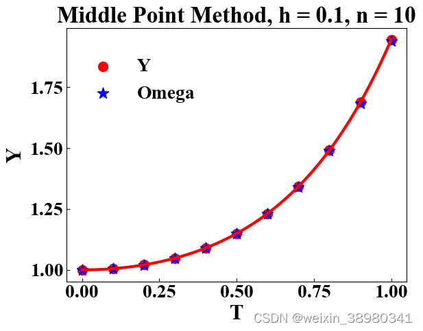
Mid-point method

$$\{\begin{array}{c}{y}^{\prime }=ty+t^3\\ y\left(0\right)=y_0\\ t\in \left[0,1\right]\end{array}$$

def func(t):  # analytical solution 
    return 3 * np.exp(np.power(t, 2)/2) - np.power(t, 2) - 2

def gf(t, y):  # gradient field
    return t * y + np.power(t, 3)

def MidpODE(t1, t2, y0, step_h=0.1, max_step=10, gf=gf):
    t = np.linspace(t1, t2, max_step + 1)
    omega = np.array([0] * (max_step + 1), dtype=float)
    omega[0] = y0
    for i in range(max_step):
        omega[i + 1] = omega[i] + step_h * gf(t[i] + step_h/2, omega[i] + step_h/2 * gf(t[i], omega[i]))
    return omega

midp_y = MidpODE(t1=0.0, t2=1.0, y0=1.0, step_h=0.1, max_step=10)

# plot:
plt.rcParams['xtick.direction'] = "in"  # ticks direction
plt.rcParams['ytick.direction'] = "in" 
axes=plt.gca()
axes.yaxis.set_major_locator(MaxNLocator(5))  # ticks num
axes.xaxis.set_major_locator(MaxNLocator(5))
plt.xticks(fontsize=20, fontweight="bold")  # ticks font
plt.yticks(fontsize=20, fontweight="bold")  
plt.xlabel("T", fontsize=22, fontweight="bold")
plt.ylabel("Y", fontsize=22, fontweight="bold")
plt.title("Middle Point Method, h = 0.1, n = 10", fontsize=24, fontweight="bold")
plt.scatter(np.linspace(0, 1, 11), func(np.linspace(0, 1, 11)), color="red", marker='o', s=100, label="Y")
plt.plot(np.linspace(0, 1, 100), func(np.linspace(0, 1, 100)), color="red", linewidth=3)
plt.scatter(np.linspace(0, 1, 11), midp_y, color="blue", marker='*', s=150, label="Omega")
# set legend:
legend_font = {
    "family": "Times New Roman", 
    "style" : "normal",
    "size" : 20, 
    'weight': "bold"
}
plt.legend(
    bbox_to_anchor=(0, 0.95), loc="upper left", 
    frameon=False, prop=legend_font
)
plt.show()

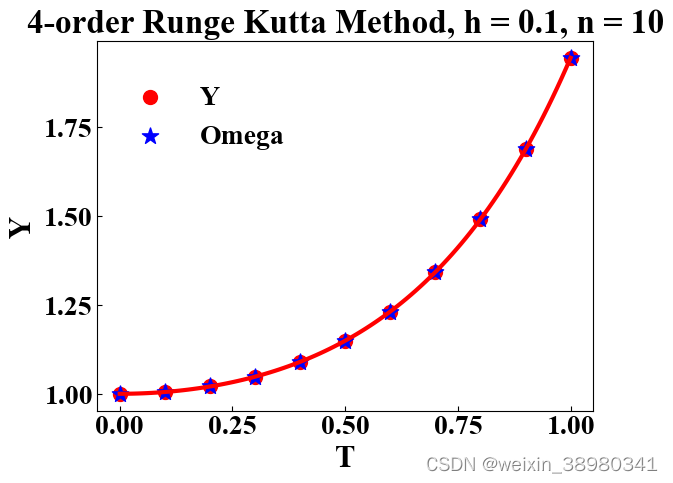
4-order Runge-Kutta method

$$\{\begin{array}{c}{y}^{\prime }=ty+t^3\\ y\left(0\right)=y_0\\ t\in \left[0,1\right]\end{array}$$

def func(t):  # analytical solution 
    return 3 * np.exp(np.power(t, 2)/2) - np.power(t, 2) - 2

def gf(t, y):  # gradient field
    return t * y + np.power(t, 3)

def RungeKutta4ODE(t1, t2, y0, step_h=0.1, max_step=10, gf=gf):
    t = np.linspace(t1, t2, max_step + 1)
    omega = np.array([0] * (max_step + 1), dtype=float)
    omega[0] = y0
    for i in range(max_step):
        s1 = gf(t[i], omega[i])
        s2 = gf(t[i] + step_h/2, omega[i] + step_h/2 * s1)
        s3 = gf(t[i] + step_h/2, omega[i] + step_h/2 * s2)
        s4 = gf(t[i] + step_h, omega[i] + step_h * s3)
        omega[i + 1] = omega[i] + step_h/6 * (s1 + 2 * s2 + 2 * s3 + s4)
    return omega

rk4_y = RungeKutta4ODE(t1=0.0, t2=1.0, y0=1.0, step_h=0.1, max_step=10)

# plot:
plt.rcParams['xtick.direction'] = "in"  # ticks direction
plt.rcParams['ytick.direction'] = "in" 
axes=plt.gca()
axes.yaxis.set_major_locator(MaxNLocator(5))  # ticks num
axes.xaxis.set_major_locator(MaxNLocator(5))
plt.xticks(fontsize=20, fontweight="bold")  # ticks font
plt.yticks(fontsize=20, fontweight="bold")  
plt.xlabel("T", fontsize=22, fontweight="bold")
plt.ylabel("Y", fontsize=22, fontweight="bold")
plt.title("4-order Runge Kutta Method, h = 0.1, n = 10", fontsize=24, fontweight="bold")
plt.scatter(np.linspace(0, 1, 11), func(np.linspace(0, 1, 11)), color="red", marker='o', s=100, label="Y")
plt.plot(np.linspace(0, 1, 100), func(np.linspace(0, 1, 100)), color="red", linewidth=3)
plt.scatter(np.linspace(0, 1, 11), rk4_y, color="blue", marker='*', s=150, label="Omega")
# set legend:
legend_font = {
    "family": "Times New Roman", 
    "style" : "normal",
    "size" : 20, 
    'weight': "bold"
}
plt.legend(
    bbox_to_anchor=(0, 0.95), loc="upper left", 
    frameon=False, prop=legend_font
)
plt.show()

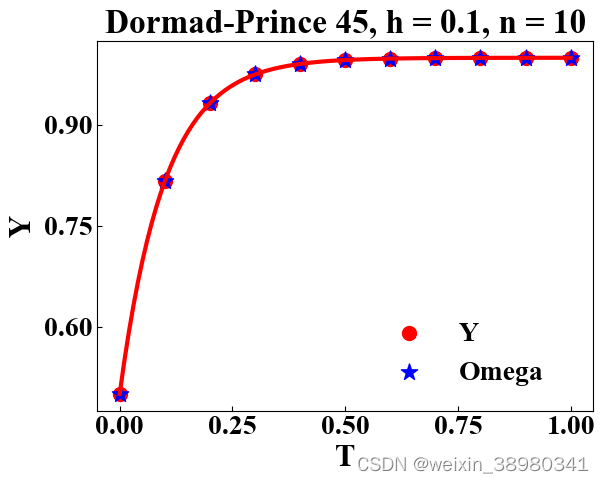
Variable step size method

Dormad-Prince 4/5

$$\{\begin{array}{c}{y}^{\prime }=10\left(1-y\right)\\ y\left(0\right)=0.5\\ t\in \left[0,100\right]\end{array}$$

def func(t):  # analytical solution 
    return 1 - np.exp(-10 * t)/2

def gf(t, y):  # gradient field
    return 10 * (1 - y)

def DormadPrince45ODE(t1, t2, y0, step_h=0.1, max_step=10, TOL=1e-4, gf=gf):
    t = np.linspace(t1, t2, max_step + 1)
    omega = np.array([0] * (max_step + 1), dtype=float)
    omega[0] = y0
    step = 1
    for i in range(max_step):
        s1 = gf(t[i], omega[i])
        s2 = gf(t[i] + step_h/5, omega[i] + step_h * 1/5 * s1)
        s3 = gf(t[i] + 3/10 * step_h, omega[i] + step_h * (3/40  * s1 + 9/40 * s2))
        s4 = gf(t[i] + 4/5 * step_h, omega[i] + step_h * (44/45 * s1 - 56/15 * s2 + 32/9 * s3))
        s5 = gf(t[i] + 8/9 * step_h, omega[i] + step_h * (19372/6561 * s1 - 25360/2187 * s2 + 64448/6561 * s3 - 212/729 * s4))
        s6 = gf(t[i] + step_h, omega[i] + step_h * (9017/3186 * s1 - 355/33 * s2 + 46732/5247 * s3 + 49/176 * s4 - 5103/18656 * s5))
        z = omega[i] + step_h * (35/384 * s1 + 500/1113 * s3 + 125/192 * s4 - 2187/6784 * s5 + 11/84 * s6)
        s7 = gf(t[i] + step_h, z)
        omega[i + 1] = omega[i] + step_h * (5179/57600 * s1 + 7571/16695 * s3 + 393/640 * s4 - 92097/339200 * s5 + 187/2100 * s6 + 1/40 * s7)
        e = step_h * np.fabs(71/57600 * s1 - 71/16695 * s3 + 71/1920 * s4 - 17253/339200 * s5 + 22/525 * s6 - 1/40 * s7)
        if e >= TOL:
            step += 1
    return omega, step

ode45_y, step = DormadPrince45ODE(t1=0.0, t2=1.0, y0=0.5, step_h = 0.1, max_step=10)
print("After {} steps, relative error less than 1e-4".format(step))

# plot:
plt.rcParams['xtick.direction'] = "in"  # ticks direction
plt.rcParams['ytick.direction'] = "in" 
axes=plt.gca()
axes.yaxis.set_major_locator(MaxNLocator(5))  # ticks num
axes.xaxis.set_major_locator(MaxNLocator(5))
plt.xticks(fontsize=20, fontweight="bold")  # ticks font
plt.yticks(fontsize=20, fontweight="bold")  
plt.xlabel("T", fontsize=22, fontweight="bold")
plt.ylabel("Y", fontsize=22, fontweight="bold")
plt.title("Dormad-Prince 45, h = 0.1, n = 10", fontsize=24, fontweight="bold")
plt.scatter(np.linspace(0, 1, 11), func(np.linspace(0, 1, 11)), color="red", marker='o', s=100, label="Y")
plt.plot(np.linspace(0, 1, 100), func(np.linspace(0, 1, 100)), color="red", linewidth=3)
plt.scatter(np.linspace(0, 1, 11), ode45_y, color="blue", marker='*', s=150, label="Omega")
# set legend:
legend_font = {
    "family": "Times New Roman", 
    "style" : "normal",
    "size" : 20, 
    'weight': "bold"
}
plt.legend(
    bbox_to_anchor=(0.95, 0), loc="lower right", 
    frameon=False, prop=legend_font
)
plt.show()