Timothy Sauer版《数值分析》学习笔记+python实现——《常微分方程》（V）【完】

Ordinary Differential Equation

Import package

import numpy as np
import matplotlib.pyplot as plt
from matplotlib.ticker import MaxNLocator
plt.rc("font", family="Times New Roman")
from tqdm import tqdm
import imageio
from mpl_toolkits.mplot3d import Axes3D

Finite difference method

Differential approximation:

$$y^{\prime }\left(t\right)\approx \frac{y\left(t+h\right)-y\left(t-h\right)}{2h}$$
$$y^{{}^{\prime \prime }}\left(t\right)\approx \frac{y\left(t+h\right)-2y\left(t\right)+y\left(t-h\right)}{h^2}$$
For boundary value problems (BVP):
$$\{\begin{array}{l}{y}^{{}^{\prime \prime }}=4y\\ y\left(0\right)=1\\ y\left(1\right)=3\end{array}$$

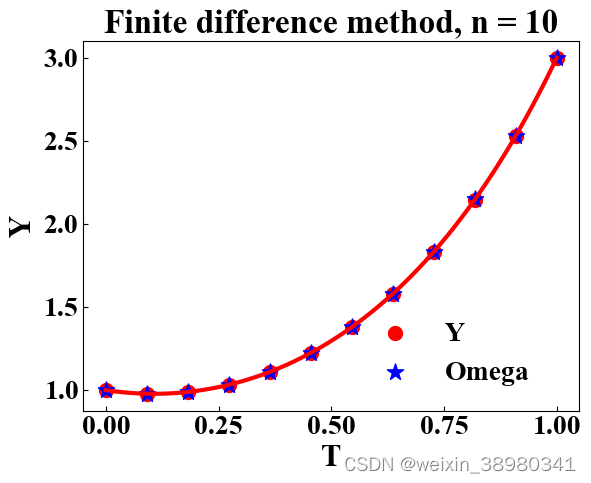
Linear BVP

The differential form of this ODE system is:
$$\frac{{\omega }_{i+1}-2{\omega }_i+{\omega }_{i-1}}{h^2}-4{\omega }_i=0⟹{\omega }_{i-1}+\left(-4h^2-2\right){\omega }_i+{\omega }_{i+1}=0$$
For the n-step Iterative method, n linear equations can be formed as follows:
$$\left(\begin{array}{ccccccc}-4h^2-2& 1& 0& \cdots & \cdots & \cdots & 0\\ 1& -4h^2-2& 1& 0& \cdots & \cdots & 0\\ 0& 1& -4h^2-2& 1& 0& \cdots & 0\\ 0& 0& \ddots & \ddots & \ddots & 0& 0\\ ⋮& ⋮& 0& 1& -4h^2-2& 1& 0\\ ⋮& ⋮& ⋮& 0& 1& -4h^2-2& 1\\ 0& 0& 0& 0& 0& 1& -4h^2-2\end{array}\right)\left(\begin{array}{l}{\omega }_1\\ {\omega }_2\\ {\omega }_3\\ ⋮\\ {\omega }_{n-2}\\ {\omega }_{n-1}\\ {\omega }_n\end{array}\right)=\left(\begin{array}{l}-1\\ 0\\ 0\\ ⋮\\ 0\\ 0\\ -3\end{array}\right)$$
Please note the appearance of boundary values, and $h=(b-a)/(n+1)$, then solve this equation groups to get: ${\omega }_0=1,{\omega }_1,\dots ,{\omega }_n,{\omega }_{n+1}=3$

# Conjugate Gradient method to solve linear equation group
def ConjugateGradient(matrix, base):
    n = len(matrix)
    x = np.array([0] * n, dtype=float)
    print("x0 = ", x.T.round(4))
    x = np.transpose([x])
    d = r = base - np.dot(matrix, x)
    rT = np.transpose(r)  # col -> row
    dT = np.transpose(d)
    for i in range(10000):
        if np.linalg.norm(r, 2) < 1e-4:
            print("Find solution: ", x.T.round(4))
            break
        rTr = np.dot(rT, r)[0, 0]  
        alpha = rTr/(np.dot(dT, np.dot(matrix, d))[0, 0])
        x = x + np.dot(alpha, d)
        print("x{} = ".format(i + 1), x.T.round(4))
        r = r - np.dot(alpha, np.dot(matrix, d))
        rT = np.transpose(r)
        beta = np.dot(rT, r)[0, 0]/rTr
        d = r + beta * d
        dT = np.transpose(d)
    return x

def func(t):  # analytical solution 
    return (3 - np.power(np.e, -2))/(np.power(np.e, 2) - np.power(np.e, -2)) * np.exp(2 * t) + (np.power(np.e, 2) - 3)/(np.power(np.e, 2) - np.power(np.e, -2)) * np.exp(-2 * t)

n_step = 10
step_h = (1.0 - 0.0)/(n_step + 1)
b_value1, b_value2 = 1.0, 3.0  # boundary value: y(0) = 1.0, y(1) = 3.0

coefficient_matrix = np.array([-4 * np.power(step_h, 2) - 2, 1] + [0] * (n_step - 2))
for i in range(1, n_step - 1):
    coefficient_matrix = np.vstack((coefficient_matrix, np.array([0] * (i - 1) + [1, -4 * np.power(step_h, 2) - 2, 1] + [0] * (n_step - 3 - (i - 1)))))
coefficient_matrix = np.vstack((coefficient_matrix, np.array([0] * (n_step - 2) + [1, -4 * np.power(step_h, 2) - 2])))
base = np.transpose([np.array([-1] + [0] * (n_step - 2) + [-3])])
omega = np.hstack((np.array([b_value1]), np.transpose(ConjugateGradient(coefficient_matrix, base)).squeeze(), np.array([b_value2])))

# plot:
plt.rcParams['xtick.direction'] = "in"  # ticks direction
plt.rcParams['ytick.direction'] = "in" 
axes=plt.gca()
axes.yaxis.set_major_locator(MaxNLocator(5))  # ticks num
axes.xaxis.set_major_locator(MaxNLocator(5))
plt.xticks(fontsize=20, fontweight="bold")  # ticks font
plt.yticks(fontsize=20, fontweight="bold")  
plt.xlabel("T", fontsize=22, fontweight="bold")
plt.ylabel("Y", fontsize=22, fontweight="bold")
plt.title("Finite difference method, n = 10", fontsize=24, fontweight="bold")
plt.scatter(np.linspace(0, 1, 12), func(np.linspace(0, 1, 12)), color="red", marker='o', s=100, label="Y")
plt.plot(np.linspace(0, 1, 100), func(np.linspace(0, 1, 100)), color="red", linewidth=3)
plt.scatter(np.linspace(0, 1, 12), omega, color="blue", marker='*', s=150, label="Omega")
# set legend:
legend_font = {
    "family": "Times New Roman", 
    "style" : "normal",
    "size" : 20, 
    'weight': "bold"
}
plt.legend(
    bbox_to_anchor=(0.95, 0), loc="lower right", 
    frameon=False, prop=legend_font
)
plt.show()

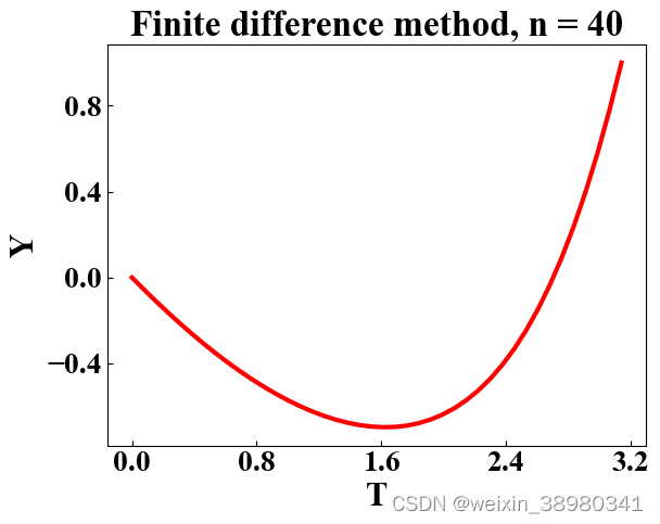
Non-linear BVP

$$\{\begin{array}{l}{y}^{{}^{\prime \prime }}=y^{\prime }+\cos y\\ y\left(0\right)=0\\ y\left(\pi \right)=1\end{array}$$
According to the finite difference method:
$$\frac{{\omega }_{i+1}-2{\omega }_i+{\omega }_{i-1}}{h^2}-\frac{{\omega }_{i+1}-{\omega }_{i-1}}{2h}-\cos {\omega }_i=0$$
$$\Rightarrow \left(1+\frac{1}{2}h\right){\omega }_{i-1}-2{\omega }_i\left(1-\frac{1}{2}h\right){\omega }_{i+1}-h^2\cos {\omega }_i=0$$
Thus, n-dimensional nonlinear functions can be obtained:
$$F\left(\omega \right)=\left(\begin{array}{c}\left(1+\frac{1}{2}h\right)y\left(a\right)-2{\omega }_i\left(1-\frac{1}{2}h\right){\omega }_2-h^2\cos {\omega }_1\\ ⋮\\ \left(1+\frac{1}{2}h\right){\omega }_{i-1}-2{\omega }_i\left(1-\frac{1}{2}h\right){\omega }_{i+1}-h^2\cos {\omega }_i\\ ⋮\\ \left(1+\frac{1}{2}h\right){\omega }_{n-1}-2{\omega }_i\left(1-\frac{1}{2}h\right)y\left(b\right)-h^2\cos {\omega }_n\end{array}\right)$$
corresponding Jacobi matrix:
$$DF\left(\omega \right)=\left(\begin{array}{ccccccc}-2+h^2\sin {\omega }_1& 1-\frac{h}{2}& 0& \cdots & \cdots & \cdots & 0\\ 1+\frac{h}{2}& -2+h^2\sin {\omega }_2& 1-\frac{h}{2}& 0& \cdots & \cdots & 0\\ 0& 1+\frac{h}{2}& -2+h^2\sin {\omega }_3& 1-\frac{h}{2}& 0& \cdots & 0\\ 0& 0& \ddots & \ddots & \ddots & 0& 0\\ ⋮& ⋮& 0& 1+\frac{h}{2}& -2+h^2\sin {\omega }_{n-2}& 1-\frac{h}{2}& 0\\ ⋮& ⋮& ⋮& 0& 1+\frac{h}{2}& -2+h^2\sin {\omega }_{n-1}& 1-\frac{h}{2}\\ 0& 0& 0& 0& 0& 1+\frac{h}{2}& -2+h^2\sin {\omega }_n\end{array}\right)$$

eps = 1e-4  
n_step = 40
step_h = (np.pi - 0.0)/(n_step + 1)  # h = (b - a)/(n + 1)
b_value1, b_value2 = 0.0, 1.0  # boundary value: y(0) = 1.0, y(1) = 3.0

def F(x, n_step, step_h):
    a = np.array([(1 + step_h/2) * b_value1 - 2 * x[0, 0] + (1 - step_h/2) * x[1, 0] - np.power(step_h, 2) * np.cos(x[0, 0])])
    b = np.array([
        [(1 + step_h/2) * x[i - 1, 0] - 2 * x[i, 0] + (1 - step_h/2) * x[i + 1, 0] - np.power(step_h, 2) * np.cos(x[i, 0])] for i in range(1, n_step -1)
    ])
    c = np.array([(1 + step_h/2) * x[n_step - 2, 0] - 2 * x[n_step - 1, 0] + (1 - step_h/2) * b_value2 - np.power(step_h, 2) * np.cos(x[n_step - 1, 0])])
    return np.vstack((a, b, c))

def DF(x, n_step, step_h): # x.size() = (n, 1)
    a = np.array([-2 + np.power(step_h, 2) * np.sin(x[0, 0]), 1 - step_h/2] + [0] * (n_step - 2), dtype=float)
    b = np.array([
        ([0] * (i - 1) + [1 + step_h/2, -2 + np.power(step_h, 2) * np.sin(x[i, 0]), 1 - step_h/2] + [0] * (n_step - 3 - (i - 1))) for i in range(1,  n_step - 1)
    ], dtype=float)
    c = np.array([0] * (n_step - 2) + [1 + step_h/2, -2 + np.power(step_h, 2) * np.sin(x[n_step - 1, 0])], dtype=float)
    return np.vstack((a, b, c))

def MultivariableNewton(n_step, step_h):  # define F(x) and DF(x) of your system first
    x = np.zeros((n_step, 1))
    last_x = np.ones((n_step, 1))
    print("x0 = ", x.T.round(4))
    i = 0
    while np.linalg.norm(x - last_x, np.inf) > eps:
        i += 1
        last_x = x
        x = x - np.dot(np.linalg.inv(DF(x, n_step=n_step,step_h=step_h)), F(x, n_step=n_step,step_h=step_h))
        print("x{} = ".format(i), x.T.round(4))
    return x

omega = np.hstack((np.array([b_value1]), np.transpose(MultivariableNewton(n_step=n_step, step_h=step_h)).squeeze(), np.array([b_value2])))

# plot:
plt.rcParams['xtick.direction'] = "in"  # ticks direction
plt.rcParams['ytick.direction'] = "in" 
axes=plt.gca()
axes.yaxis.set_major_locator(MaxNLocator(5))  # ticks num
axes.xaxis.set_major_locator(MaxNLocator(5))
plt.xticks(fontsize=20, fontweight="bold")  # ticks font
plt.yticks(fontsize=20, fontweight="bold")  
plt.xlabel("T", fontsize=22, fontweight="bold")
plt.ylabel("Y", fontsize=22, fontweight="bold")
plt.title("Finite difference method, n = 40", fontsize=24, fontweight="bold")
plt.plot(np.linspace(0, np.pi, n_step + 2), omega, color="red", linewidth=3)
# set legend:
legend_font = {
    "family": "Times New Roman", 
    "style" : "normal",
    "size" : 20, 
    'weight': "bold"
}
plt.legend(
    bbox_to_anchor=(0.95, 0), loc="lower right", 
    frameon=False, prop=legend_font
)
plt.show()

Collocation and Finite element method

The solution is given a functional form whose parameters are fit by the method.
Choose a set of basis functions ${\varphi }_1(t),\dots ,{\varphi }_n(t)$, which may be polynomials, trigonometric functions, splines, or other simple functions. Then consider the possible solution:
$$y\left(t\right)=\sum _{i=1}^n{c}_i{\varphi }_i\left(t\right)$$

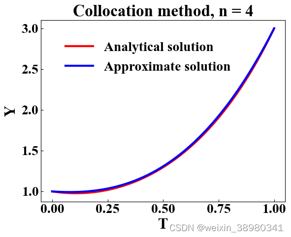
Collocation method

For BVP:
$$\{\begin{array}{l}{y}^{{}^{\prime \prime }}=f\left(t,y,y^{\prime }\right)\\ y\left(a\right)=y_a\\ y\left(b\right)=y_b\end{array}$$
Choose n points, beginning and ending with the boundary points $a$ and $b$, say:
$$a=t_1<\cdots <t_n=b$$
Here, we choose the basis functions ${\varphi }_j(t)=t^{j-1}$ for $1⩽j⩽n$. The solution will be of form：
$$y\left(t\right)=\sum _{j=1}^n{c}_j{\varphi }_j\left(t\right)=\sum _{j=1}^n{c}_i{t}^{j-1}$$
We will write n equations in the $n$ unknowns $c_1,...,c_n$. The first and last are the boundary conditions:
$$\begin{gathered} i=1:\sum _{j=1}^n{c}_j{a}^{j-1}=y\left(a\right) \\ i=n:\sum _{j=1}^n{c}_j{b}^{j-1}=y\left(b\right) \end{gathered}$$
The remaining $n-2$ equations come from the differential equation evaluated at $t_i$ for $2⩽i⩽n-1$:
$$\sum _{j=1}^n\left(j-1\right)\left(j-2\right)c_j{t}^{j-3}=f\left(t,\sum _{j=1}^n{c}_j{t}^{j-1},\sum _{j=1}^n\left(j-1\right)c_j{t}^{j-2}\right)$$

Application

For BVP:
$$\{\begin{array}{l}{y}^{{}^{\prime \prime }}=4y\\ y\left(0\right)=1\\ y\left(1\right)=3\end{array}$$
Through collocation method:
$$i=1:\sum _{j=1}^n{c}_j{a}^{j-1}=c_1=1$$
$$i=n:\sum _{j=1}^n{c}_j{b}^{j-1}=\sum _{j=1}^n{c}_j=3$$
$$\begin{gathered} \sum _{j=1}^n\left(j-1\right)\left(j-2\right)c_j{t}_i^{j-3}=f\left(t,\sum _{j=1}^n{c}_j{t}_i^{j-1},\sum _{j=1}^n\left(j-1\right)c_j{t}_i^{j-2}\right) \\ \Rightarrow \sum _{j=1}^n\left[\left(j-1\right)\left(j-2\right)c_j{t}_i^{j-3}-4t_i^{j-1}\right]c_j=0 \end{gathered}$$
which gives us a n-dimension linear equation:
$$\left(\begin{array}{ccccc}1& 0& \cdots & \cdots & 0\\ \cdots & \cdots & \left(j-1\right)\left(j-2\right)t_i^{j-3}-4t_i^{j-1}& \cdots & \cdots \\ 1& 1& \cdots & \cdots & 1\end{array}\right)\left(\begin{array}{c}{c}_1\\ ⋮\\ c_n\end{array}\right)=\left(\begin{array}{c}1\\ ⋮\\ 3\end{array}\right);1⩽j⩽n,2⩽i⩽n-1$$
where:$t_i=a+\frac{i-1}{n-1}\left(b-a\right)=\frac{i-1}{n-1}$

def Householder(matrix):
    A = np.transpose(matrix)
    n = A.shape[1]
    omega = np.array([np.linalg.norm(A[0], 2)] + [0] * (n - 1))
    v = omega - A[0]
    P = np.dot(np.transpose([v]), [v])/np.dot([v], np.transpose([v]))
    H_hat = np.eye(n) - 2 * P
    return H_hat

def AugmentH(h_hat, n):
    r = n - len(h_hat)
    return np.block([
            [np.eye(r, r), np.zeros((r, len(h_hat)))], 
            [np.zeros((len(h_hat), r)), h_hat]
    ])

def HouseholderQRDecomposition(matrix):
    A = np.transpose(matrix)
    hid_r = np.eye(len(matrix))
    state = matrix
    for i in range(matrix.shape[1]):
        h_hat = Householder(state)
        H = AugmentH(h_hat, len(matrix))
        hid_r = np.dot(H, hid_r)
        state = np.dot(hid_r, matrix)
        state = state[i + 1:, i + 1:]
        if state.shape[0] < 2:
            break
        cnt = 0
        for i in range(1, state.shape[0]):
            if state[i][0] == 0:
                cnt += 1  
        if cnt == state.shape[0] - 1:
            break
    R = np.dot(hid_r, matrix)
    Q = np.linalg.inv(hid_r)
    return Q, R

def GaussSeidel(matrix, base):
    x = np.array([0] * len(base))
    print("x0 = ", x.round(4))
    x = np.transpose([x])
    D = np.diag(np.diag(matrix))
    L = np.tril(matrix)
    U = np.triu(matrix) - D
    L_i = np.linalg.inv(L)
    i = 1
    while np.linalg.norm((base - np.dot(matrix, x)), np.inf) > eps:
        x = np.dot(L_i, (base - np.dot(U, x)))
        print("x{} = ".format(i), x.T.round(4))
        i += 1
    return x

def func(t):  # analytical solution 
    return (3 - np.power(np.e, -2))/(np.power(np.e, 2) - np.power(np.e, -2)) * np.exp(2 * t) + (np.power(np.e, 2) - 3)/(np.power(np.e, 2) - np.power(np.e, -2)) * np.exp(-2 * t)

def phi(t, cs):  # discrete function
    if isinstance(t, np.ndarray):
        ret = np.array([0] * len(t), dtype=float)
    else:
        ret = 0
    for i in range(len(cs)):
        ret += cs[i] * np.power(t, i)
    return ret

n_step = 4
t = [(i - 1)/(n_step - 1) for i in range(2, n_step)]
a = np.array([1] + [0] * (n_step - 1), dtype=float)
b = np.array([
    [(j - 1) * (j - 2) * np.power(((i - 1)/(n_step - 1)), j - 3) - 4 * np.power(((i - 1)/(n_step - 1)), j - 1) for j in range(1, n_step + 1)] for i in range(2, n_step)
], dtype=float) 
c = np.array([1] * n_step, dtype=float)
if n_step > 2:
    coefficient_matrix = np.vstack((a, b, c))
else:
    coefficient_matrix = np.vstack((a, c))
base = np.transpose([np.array([1] + (n_step - 2) * [0] + [3], dtype=float)])
Q, R = HouseholderQRDecomposition(coefficient_matrix)
R_hat = R[:n_step, :n_step]
d_hat = np.dot(np.transpose(Q), base)[:n_step, :]
cs = GaussSeidel(matrix=R_hat, base=d_hat)

# plot:
plt.rcParams['xtick.direction'] = "in"  # ticks direction
plt.rcParams['ytick.direction'] = "in" 
axes=plt.gca()
axes.yaxis.set_major_locator(MaxNLocator(5))  # ticks num
axes.xaxis.set_major_locator(MaxNLocator(5))
plt.xticks(fontsize=20, fontweight="bold")  # ticks font
plt.yticks(fontsize=20, fontweight="bold")  
plt.xlabel("T", fontsize=22, fontweight="bold")
plt.ylabel("Y", fontsize=22, fontweight="bold")
plt.title("Collocation method, n = 4", fontsize=24, fontweight="bold")
plt.plot(np.linspace(0, 1, 100), func(np.linspace(0, 1, 100)), color="red", linewidth=3, label="Analytical solution")
plt.plot(np.linspace(0, 1, 100), phi(np.linspace(0, 1, 100), cs), color="blue", linewidth=3, label="Approximate solution")
# set legend:
legend_font = {
    "family": "Times New Roman", 
    "style" : "normal",
    "size" : 20, 
    'weight': "bold"
}
plt.legend(
    bbox_to_anchor=(0.05, 0.95), loc="upper left", 
    frameon=False, prop=legend_font
)
plt.show()

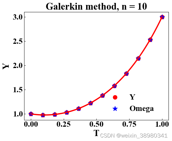
Galerkin method (finite element analysis)

The choice of splines as basis functions leads to the Finite Element Method as:
$$y\left(t\right)=\sum _{j=0}^{n+1}{c}_j{\varphi }_j(t)$$
$${\varphi }_i\left(t\right)=\{\begin{array}{l}\frac{t-t_{i-1}}{t_i-t_{i-1}};when{t}_{i-1}<t⩽t_i\\ \frac{t_{i+1}-t}{t_{i+1}-t_i};when{t}_i<t⩽t_{i+1}\\ 0;other\end{array}$$
$${\varphi }_0\left(t\right)=\{\begin{array}{l}\frac{t_1-t}{t_1-t_0};when{t}_0<t⩽t_1\\ 0;other\end{array};{\varphi }_{n+1}\left(t\right)=\{\begin{array}{l}\frac{t-t_n}{t_{n+1}-t_n};when{t}_n<t⩽t_{n+1}\\ 0;other\end{array}$$
The piecewise-linear “tent” functions ${\varphi }_i(t)$ has the following properties:
$${\varphi }_i\left(j\right)={\delta }_{ij}$$
$$\sum _{i=0}^{n+1}{c}_i{\varphi }_i\left(t\right)=c_j$$
$${\int }_a^b{\varphi }_i\left(t\right){\varphi }_{i+1}\left(t\right)dt=\frac{h}{6};{\int }_a^b{\left[{\varphi }_i\left(t\right)\right]}^{2}dt=\frac{2h}{3}$$
$${\int }_a^b{\varphi }_i\left(t\right){\varphi }_{i+1}^{\prime }\left(t\right)dt=-\frac{1}{h};{\int }_a^b{\left[{\varphi }_i^{\prime }\left(t\right)\right]}^{2}dt=\frac{2}{h}$$
where $h$ is the time step.

For BVP:
$$\{\begin{array}{l}{y}^{{}^{\prime \prime }}=f\left(t,y,y^{\prime }\right)\\ y\left(a\right)=y_a\\ y\left(b\right)=y_b\end{array}$$
The Galerkin Method consists of two main ideas. The first is to minimize $r$ by
forcing it to be orthogonal to the basis functions:
$${\int }_a^b{y}^{{}^{\prime \prime }}\left(t\right){\varphi }_i\left(t\right)dt={\int }_a^b{f}^{\prime }\left(t,y,y^{\prime }\right){\varphi }_i\left(t\right)dt$$
Now apply integration by parts to eliminate the second derivatives:
$${\int }_a^b{y}^{{}^{\prime \prime }}\left(t\right){\varphi }_i\left(t\right)dt={\varphi }_i\left(b\right)y^{\prime }\left(b\right)-{\varphi }_i\left(a\right)y^{\prime }\left(a\right)-{\int }_a^b{y}^{\prime }\left(t\right){\varphi }_i^{\prime }\left(t\right)dt$$
According the properties of tent functions:
$$y\left(a\right)=\sum _{i=0}^{n+1}{c}_i{\varphi }_i\left(a\right)=\sum _{i=0}^{n+1}{c}_i{\varphi }_i\left(t_0\right)=c_0$$
$$y\left(b\right)=\sum _{i=0}^{n+1}{c}_i{\varphi }_i\left(b\right)=\sum _{i=0}^{n+1}{c}_i{\varphi }_i\left(t_{n+1}\right)=c_{n+1}$$
Therefore, the integration formula can be written as ($i=1,\dots ,n$):
$${\int }_a^{b}f\left(t,y,y^{\prime }\right){\varphi }_i\left(t\right)dt+{\int }_a^b{y}^{\prime }\left(t\right){\varphi }_i^{\prime }\left(t\right)dt=0$$

Application

For BVP:
$$\{\begin{array}{l}{y}^{{}^{\prime \prime }}=4y\\ y\left(0\right)=1\\ y\left(1\right)=3\end{array}$$
Through collocation method:
$$\sum _{j=0}^{n+1}{c}_j\left[4{\int }_0^1{\varphi }_i\left(t\right){\varphi }_j\left(t\right)dt+{\int }_0^1{\varphi }_j^{\prime }\left(t\right){\varphi }_i^{\prime }\left(t\right)dt\right]$$
System of linear equations can be obtained:
$$\left(\begin{array}{ccccccc}\alpha & \beta & 0& \cdots & \cdots & \cdots & 0\\ \beta & \alpha & \beta & 0& \cdots & \cdots & 0\\ 0& \beta & \alpha & \beta & 0& \cdots & 0\\ 0& 0& \ddots & \ddots & \ddots & 0& 0\\ ⋮& ⋮& 0& \beta & \alpha & \beta & 0\\ ⋮& ⋮& ⋮& 0& \beta & \alpha & \beta \\ 0& 0& 0& 0& 0& \beta & \alpha \end{array}\right)\left(\begin{array}{c}{c}_1\\ ⋮\\ ⋮\\ ⋮\\ ⋮\\ ⋮\\ c_n\end{array}\right)=\left(\begin{array}{c}-y_a\beta \\ 0\\ ⋮\\ ⋮\\ ⋮\\ 0\\ -y_b\beta \end{array}\right)$$
where
$$\alpha =\frac{8}{3}h+\frac{2}{h};\beta =\frac{2}{3}h-\frac{1}{h};y_a=1;y_b=3$$

def func(t):  # analytical solution 
    return (3 - np.power(np.e, -2))/(np.power(np.e, 2) - np.power(np.e, -2)) * np.exp(2 * t) + (np.power(np.e, 2) - 3)/(np.power(np.e, 2) - np.power(np.e, -2)) * np.exp(-2 * t)

n_step = 10
step_h = (1.0 - 0.0)/(n_step + 1)
b_value1, b_value2 = 1.0, 3.0  # boundary value: y(0) = 1.0, y(1) = 3.0
alpha = 8/3 * step_h + 2/step_h
beta = 2/3 * step_h - 1/step_h
a = np.array([alpha, beta] + [0] * (n_step - 2), dtype=float)
b = np.array([
    ([0] * (i - 1) + [beta, alpha, beta] + [0] * (n_step - 3 - (i - 1))) for i in range(1, n_step - 1)
])
c = np.array([0] * (n_step - 2) + [beta, alpha], dtype=float)
if n_step > 2:
    coefficient_matrix = np.vstack((a, b, c))
else:
    coefficient_matrix = np.vstack((a, c))
base = np.transpose([np.array([-b_value1 * beta] + [0] * (n_step - 2) + [-b_value2 * beta], dtype=float)])
omega = np.hstack((np.array([b_value1]), np.transpose(GaussSeidel(matrix=coefficient_matrix, base=base)).squeeze(), np.array([b_value2])))

# plot:
plt.rcParams['xtick.direction'] = "in"  # ticks direction
plt.rcParams['ytick.direction'] = "in" 
axes=plt.gca()
axes.yaxis.set_major_locator(MaxNLocator(5))  # ticks num
axes.xaxis.set_major_locator(MaxNLocator(5))
plt.xticks(fontsize=20, fontweight="bold")  # ticks font
plt.yticks(fontsize=20, fontweight="bold")  
plt.xlabel("T", fontsize=22, fontweight="bold")
plt.ylabel("Y", fontsize=22, fontweight="bold")
plt.title("Galerkin method, n = 10", fontsize=24, fontweight="bold")
plt.scatter(np.linspace(0, 1, 12), func(np.linspace(0, 1, 12)), color="red", marker='o', s=100, label="Y")
plt.plot(np.linspace(0, 1, 100), func(np.linspace(0, 1, 100)), color="red", linewidth=3)
plt.scatter(np.linspace(0, 1, 12), omega, color="blue", marker='*', s=150, label="Omega")
# set legend:
legend_font = {
    "family": "Times New Roman", 
    "style" : "normal",
    "size" : 20, 
    'weight': "bold"
}
plt.legend(
    bbox_to_anchor=(0.95, 0), loc="lower right", 
    frameon=False, prop=legend_font
)
plt.show()