python minimize_同义词词向量训练python实现

Boblee人工智能硕士毕业，擅长及爱好python，基于python研究人工智能、群体智能、区块链等技术，并使用python开发前后端、爬虫等。

本文基于https://zhuanlan.zhihu.com/p/28979653进行修改。

1. word2vec简要介绍

      word2vec 是 Google 于 2013 年开源推出的一个用于获取 word vector 的工具包，它简单、高效，因此引起了很多人的关注。对word2vec数学原理感兴趣的可以移步word2vec 中的数学原理详解，这里就不具体介绍。word2vec对词向量的训练有两种方式，一种是CBOW模型，即通过上下文来预测中心词；另一种skip-Gram模型，即通过中心词来预测上下文。其中CBOW对小型数据比较适合，而skip-Gram模型在大型的训练语料中表现更好。

   2.  同义词训练

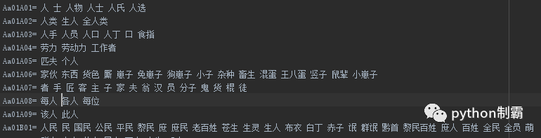
     本文基于哈工大提供的同义词词林进行训练，数据集请见：      https://github.com/TernenceWind/replaceSynbycilin

     本文训练采取以下步骤：

    1. 提取同义词将所有词组成一个列表，为构建词频统计，词典及反转词典。因为计算机不能理解中文，我们必须把文字转换成数值来替代。

   2.构建训练集，每次随机选择一行同义词，比如选取“人类、主人、全人类”这一行，输入“人类”预测“主人”，输入“主人”预测“全人类”。

3.python实现

初始化数据

from __future__ import absolute_importfrom __future__ import divisionfrom __future__ import print_functionfrom random import choiceimport collectionsimport mathimport randomimport numpy as npfrom six.moves import xrangeimport tensorflow as tfdata = []all_word = []for line in open('cilin.txt', 'r', encoding='utf8'):    line =  line.replace('\n','').split(' ')[1:]    # line  =line.strip('\n')    # line = line.split(' ')    data.append(line)    for element in line:        if element not in all_word:            all_word.append(element)dictionary = [i for i in range(len(all_word))]reverse_dictionary_ = dict(zip(dictionary, all_word))reverse_dictionary = dict(zip(all_word, dictionary))

获取训练集

batch_size = 128embedding_size = 128skip_window = 1num_skips = 2valid_size = 4    valid_window = 100num_sampled = 64   vocabulary_size  =len(all_word)#验证集valid_word = ['专家','住户','祖父','家乡']valid_examples =[reverse_dictionary[li] for li in valid_word]def generate_batch(data,batch_size):    data_input = np.ndarray(shape=(batch_size), dtype=np.int32)    data_label = np.ndarray(shape=(batch_size, 1), dtype=np.int32)    for i in range(batch_size):        slice = random.sample( choice(data), 2)        data_input[i ] = reverse_dictionary[slice[0]]        data_label[i , 0] = reverse_dictionary[slice[1]]    return data_input, data_label

构建网络

graph = tf.Graph()with graph.as_default():    # Input data.    train_inputs = tf.placeholder(tf.int32, shape=[batch_size])    train_labels = tf.placeholder(tf.int32, shape=[batch_size, 1])    valid_dataset = tf.constant(valid_examples, dtype=tf.int32)    # Ops and variables pinned to the CPU because of missing GPU implementation    with tf.device('/cpu:0'):        # Look up embeddings for inputs.        embeddings = tf.Variable(            tf.random_uniform([vocabulary_size, embedding_size], -1.0, 1.0))        embed = tf.nn.embedding_lookup(embeddings, train_inputs)        # Construct the variables for the NCE loss        nce_weights = tf.Variable(            tf.truncated_normal([vocabulary_size, embedding_size],                                stddev=1.0 / math.sqrt(embedding_size)))        nce_biases = tf.Variable(tf.zeros([vocabulary_size]),dtype=tf.float32)    # Compute the average NCE loss for the batch.    # tf.nce_loss automatically draws a new sample of the negative labels each    # time we evaluate the loss.    loss = tf.reduce_mean(tf.nn.nce_loss(weights=nce_weights,                                         biases=nce_biases,                                         inputs=embed,                                         labels=train_labels,                                         num_sampled=num_sampled,                                         num_classes=vocabulary_size))    # Construct the SGD optimizer using a learning rate of 1.0.    optimizer = tf.train.GradientDescentOptimizer(1.0).minimize(loss)    # Compute the cosine similarity between minibatch examples and all embeddings.    norm = tf.sqrt(tf.reduce_sum(tf.square(embeddings), 1, keep_dims=True))    normalized_embeddings = embeddings / norm    valid_embeddings = tf.nn.embedding_lookup(normalized_embeddings, valid_dataset)    similarity = tf.matmul(valid_embeddings, normalized_embeddings, transpose_b=True)    # Add variable initializer.    init = tf.global_variables_initializer()

开始训练

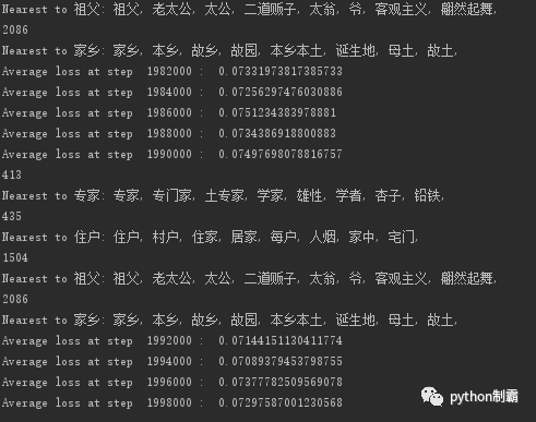
num_steps = 2000000with tf.Session(graph=graph) as session:    # We must initialize all variables before we use them.    init.run()    print("Initialized")    average_loss = 0    for step in xrange(num_steps):        batch_inputs, batch_labels = generate_batch(data,batch_size)        feed_dict = {train_inputs: batch_inputs, train_labels: batch_labels}        # We perform one update step by evaluating the optimizer op (including it        # in the list of returned values for session.run()        _, loss_val = session.run([optimizer, loss], feed_dict=feed_dict)        average_loss += loss_val        if step % 2000 == 0:            if step > 0:                average_loss /= 2000            # The average loss is an estimate of the loss over the last 2000 batches.            print("Average loss at step ", step, ": ", average_loss)            average_loss = 0        # Note that this is expensive (~20% slowdown if computed every 500 steps)        if step % 10000 == 0:            sim = similarity.eval()            for i in xrange(valid_size):                print(valid_examples[i])                valid_word = reverse_dictionary_[valid_examples[i]]                top_k = 8  # number of nearest neighbors                nearest = (-sim[i, :]).argsort()[:top_k]                log_str = "Nearest to %s:" % valid_word                for k in xrange(top_k):                    close_word = reverse_dictionary_[nearest[k]]                    log_str = "%s %s," % (log_str, close_word)                print(log_str)    final_embeddings = normalized_embeddings.eval()    np.save('tongyi.npy',final_embeddings)

可视化

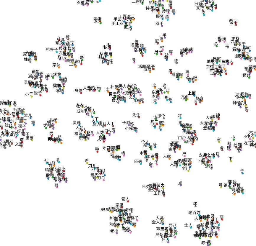
def plot_with_labels(low_dim_embs, labels, filename='images/tsne3.png',fonts=None):    assert low_dim_embs.shape[0] >= len(labels), "More labels than embeddings"    plt.figure(figsize=(15, 15))  # in inches    for i, label in enumerate(labels):        x, y = low_dim_embs[i, :]        plt.scatter(x, y)        plt.annotate(label,                    fontproperties=fonts,                    xy=(x, y),                    xytext=(5, 2),                    textcoords='offset points',                    ha='right',                    va='bottom')    plt.savefig(filename,dpi=800)try:    from sklearn.manifold import TSNE    import matplotlib.pyplot as plt    from matplotlib.font_manager import FontProperties    font = FontProperties(fname=r"simhei.ttf", size=14)    tsne = TSNE(perplexity=30, n_components=2, init='pca', n_iter=5000)    plot_only = 100    low_dim_embs = tsne.fit_transform(final_embeddings[:plot_only, :])    labels = [reverse_dictionary_[i] for i in xrange(plot_only)]    plot_with_labels(low_dim_embs, labels,fonts=font)except ImportError:    print("Please install sklearn, matplotlib, and scipy to visualize embeddings.")

4.实验结果

训练结果

从图中可见 同义词基本训练出来了。

5.结语

     本文基于前人的基础上实现了同义词词向量生成，下一步就可以用于nlp文本处理了。