三种页面置换算法c语言代码_三种梯度下降算法及代码实现

三种梯度下降算法及代码实现

• 批量梯度下降算法(Batch Gradient Descent)
• 随机梯度下降法（Stochastic gradient descent, SGD）
• 小批量梯度下降（Mini-Batch Gradient Descent, MBGD）

我们先创建一组数据，来对这组数据应用一下三种梯度下降看下区别。
我们在python里面实现可视化，首先需要导入一些必要的包
import numpy as np import os %matplotlib inline import matplotlib.pyplot as plt #画图包
然后，我们自己创建参数来在python中实现三种算法
#随机种子 np.random.seed(42) #保存图像 PROJECT_ROOT_DIR = '.' MODEL_ID = 'linear_modele' def save_fig(fig_id,tight_lavout = True):#定义一个保存图像的函数 #制定保存图像的路径，当前目录下的images文件夹下的model_id文件夹 path = os.path.join(PROJECT_ROOT_DIR,'images',MODEL_ID,fig_id+'.png') print('Saving figure',fig_id)#提示函数，正在保存图片 plt.savefig(path,format = 'png',dpi = 300)#保存图片（指定保存路径，格式，图像分辨率） #去掉警告 import warnings warnings.filterwarnings(action = 'ignore',message = 'interna #模拟x数据与y数据 x = 2*np.random.rand(100,1) y = 4+3*x +np.random.randn(100,1)
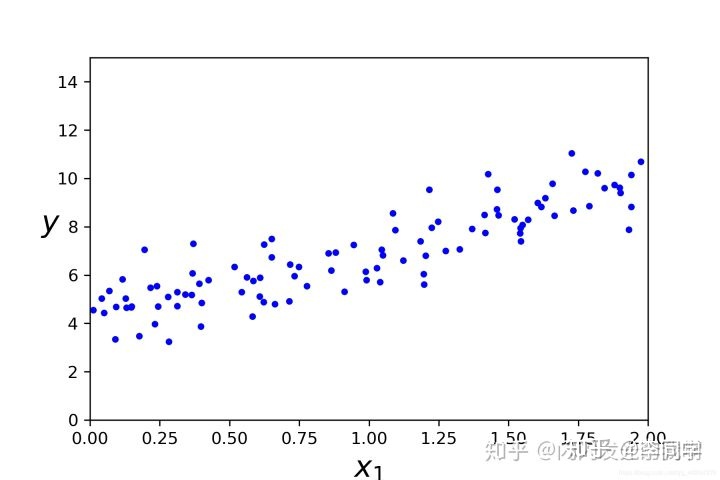
这种代码我们并不能直观的感受到我们所写的数据，我们可以通过在python中绘图的方式来直观体现。
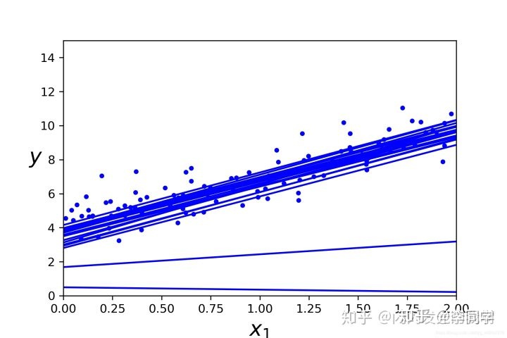
#画图 plt.plot(x,y,'b.') plt.xlabel('$x_1$',fontsize=18) plt.ylabel('$y$',rotation = 0,fontsize=18) plt.axis([0,2,0,15]) save_fig('generated_data_plot')#保存图片 plt.show()

导包做预测：
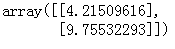
# 添加新特征 X_b = np.c_[np.ones((100,1)),X] # 创建测试数据 X_new=np.array([[0],[2]]) X_new_b=np.c_[np.ones((2,1)),X_new] # 从sklearn 包里导入线性回归方程 from sklearn.linear_model import LinearRegression lin_reg=LinearRegression() #创建线性回归对象 lin_reg.fit(X,y) #拟合训练数据 lin_reg.intercept_,lin_reg.coef_ #输出截距,斜率

# 对测试集进行预测 lin_reg.predict(X_new)

1. 批量梯度下降算法(Batch Gradient Descent)

指在计算梯度下降的每一步中，我们都用到了所有的训练样本，在梯度下降中，在计算微积分时，我们需要进行求和运算。
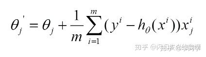
上篇文章介绍过，批量梯度下降中的更新过程如下：

代码实现：
eta = 0.1 #学习率 n_iterations = 1000 #迭代次数 m = 100 #训练集中实例的数量 theta = np.random.randn(2,1) #参数值 for iteration in range(n_iterations):# 限定迭代次数 gradients = 2/m * X_b.T.dot(X_b.dot(theta) - y) #梯度 theta = theta - eta * gradients #更新theta
定义一个函数来实现不同的参数，学习率对算法的影响
theta_path_bgd = [] def plot_gradient_descent(theta, eta, theta_path=None): m = len(X_b) plt.plot(X, y, "b.") n_iterations = 1000 for iteration in range(n_iterations): if iteration < 10: y_predict = X_new_b.dot(theta) style = "b-" plt.plot(X_new, y_predict, style) gradients = 2/m * X_b.T.dot(X_b.dot(theta) - y) theta = theta - eta * gradients if theta_path is not None: theta_path.append(theta) plt.xlabel("$x_1$", fontsize=18) plt.axis([0, 2, 0, 15]) plt.title(r"$eta = {}$".format(eta), fontsize=16)
通过图示的方式来展现一下不同的学习率对算法的影响
np.random.seed(42) theta = np.random.randn(2,1) plt.figure(figsize=(10,4)) plt.subplot(131); plot_gradient_descent(theta, eta=0.02) plt.ylabel("$y$", rotation=0, fontsize=18) plt.subplot(132); plot_gradient_descent(theta, eta=0.1, theta_path=theta_path_bgd) plt.subplot(133); plot_gradient_descent(theta, eta=0.5) save_fig("gradient_descent_plot") plt.show()

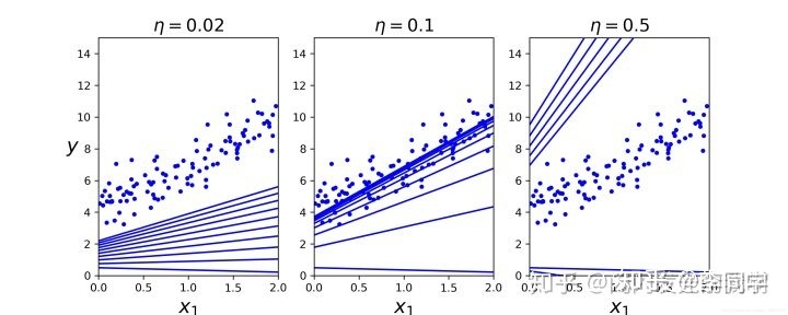
从图中可以观察得到，学习率取得过小时，多次都找不到最小值，步伐太小了，迟迟接近不了；学习率过大时，容易跳过最小值，步子过大，直接跨到后面。可见，取得一个适中的学习率是非常重要的。
2. 随机梯度下降法（Stochastic gradient descent, SGD）
随机梯度下降是通过每个样本来迭代更新一次，一次迭代不可能最优，如果迭代10次的话就需要遍历训练样本10次。
与批量梯度下降算法的代码类似
theta_path_sgd = [] m = len(X_b) np.random.seed(42) n_epochs = 50 theta = np.random.randn(2,1) # 随机初始化 for epoch in range(n_epochs): for i in range(m): if epoch == 0 and i < 20: y_predict = X_new_b.dot(theta) style = "b-" plt.plot(X_new, y_predict, style) # random_index = np.random.randint(m) xi = X_b[i:i+1] yi = y[i:i+1] gradients = 2 * xi.T.dot(xi.dot(theta) - yi) eta = 0.1 theta = theta - eta * gradients theta_path_sgd.append(theta)
同样我们可以用图来看一下此算法
plt.plot(X, y, "b.") plt.xlabel("$x_1$", fontsize=18) plt.ylabel("$y$", rotation=0, fontsize=18) plt.axis([0, 2, 0, 15]) save_fig("sgd_plot") plt.show()

3. 小批量梯度下降（Mini-Batch Gradient Descent, MBGD）
小批量梯度下降法是为了解决批梯度下降法的训练速度慢，以及随机梯度下降法的准确性综合而来。
代码实现：
theta_path_mgd = [] n_iterations = 50 minibatch_size = 20 np.random.seed(42) theta = np.random.randn(2,1) # random initialization for epoch in range(n_iterations): shuffled_indices = np.random.permutation(m) X_b_shuffled = X_b[shuffled_indices] y_shuffled = y[shuffled_indices] for i in range(0, m, minibatch_size): xi = X_b_shuffled[i:i+minibatch_size] yi = y_shuffled[i:i+minibatch_size] gradients = 2/minibatch_size * xi.T.dot(xi.dot(theta) - yi) eta = 0.1 theta = theta - eta * gradients theta_path_mgd.append(theta)
此时，我们三种算法已经写完，我们可以把它放在一张图上来比较一下，进行总结
theta_path_bgd = np.array(theta_path_bgd) theta_path_sgd = np.array(theta_path_sgd) theta_path_mgd = np.array(theta_path_mgd) plt.figure(figsize=(7,4)) plt.plot(theta_path_sgd[:,0], theta_path_sgd[:,1], "r-s", linewidth=1, label="Stochastic") plt.plot(theta_path_mgd[:,0], theta_path_mgd[:,1], "g-+", linewidth=2, label="Mini-batch") plt.plot(theta_path_bgd[:,0], theta_path_bgd[:,1], "b-o", linewidth=3, label="Batch") plt.legend(loc = "upper left",fontsize=16) plt.xlabel(r"$theta_0$",fontsize=20) plt.ylabel(r"$theta_1$",fontsize=20,rotation=0) plt.axis([2.5,4.5,2.3,3.9]) save_fig("gradient_descent_plaths_plot") plt.show()

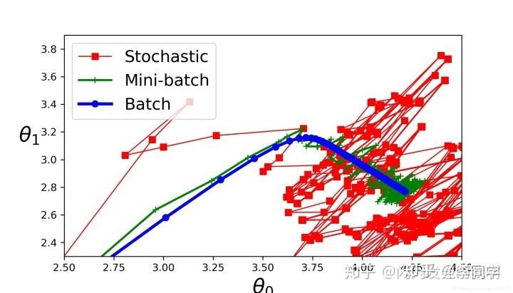
我们可以直观的感受到这三种类型的梯度下降算法的差别：小批量梯度下降法解决了批量梯度下降的训练速度慢的问题，并且解决来随机梯度下降法的准确性的问题。