python datasets 下载_使用python+sklearn实现在小型数据集上比较不同的层次链接方法...

注意：单击此处https://urlify.cn/NV3Erq下载完整的示例代码，或通过Binder在浏览器中运行此示例

此示例显示了在二维模式下的数据集上层次聚类(hierarchical clustering)的不同链接方法的特征。 主要观察到的有：

• 单链接的速度很快，并且可以在非球形数据上表现良好，但是在存在噪声的情况下，效果表现较差。
• 平均链接和完全链接在分离干净的球状上表现良好，但在其他方面却有不同的结果。
• Ward是处理有噪声数据的最有效方法。

尽管这些示例给出了有关算法的一些信息，但这种信息可能不适用于非常高维的数据。

print(__doc__)import timeimport warningsimport numpy as npimport matplotlib.pyplot as pltfrom sklearn import cluster, datasetsfrom sklearn.preprocessing import StandardScalerfrom itertools import cycle, islicenp.random.seed(0)

生成数据集：我们选择足够大的样本数量以查看算法的可扩展性，但又不能设置太大，以避免运行时间太长。

n_samples = 1500noisy_circles = datasets.make_circles(n_samples=n_samples, factor=.5,                                      noise=.05)noisy_moons = datasets.make_moons(n_samples=n_samples, noise=.05)blobs = datasets.make_blobs(n_samples=n_samples, random_state=8)no_structure = np.random.rand(n_samples, 2), None# 各向异性(Anisotropicly)分布的数据random_state = 170X, y = datasets.make_blobs(n_samples=n_samples, random_state=random_state)transformation = [[0.6, -0.6], [-0.4, 0.8]]X_aniso = np.dot(X, transformation)aniso = (X_aniso, y)# 具有变化的斑点(blobs)varied = datasets.make_blobs(n_samples=n_samples,                             cluster_std=[1.0, 2.5, 0.5],                             random_state=random_state)

运行聚类并绘图

# 设置聚类参数plt.figure(figsize=(9 * 1.3 + 2, 14.5))plt.subplots_adjust(left=.02, right=.98, bottom=.001, top=.96, wspace=.05,                    hspace=.01)plot_num = 1default_base = {'n_neighbors': 10,                'n_clusters': 3}datasets = [    (noisy_circles, {'n_clusters': 2}),    (noisy_moons, {'n_clusters': 2}),    (varied, {'n_neighbors': 2}),    (aniso, {'n_neighbors': 2}),    (blobs, {}),    (no_structure, {})]for i_dataset, (dataset, algo_params) in enumerate(datasets):    # 使用数据集特定的值更新参数    params = default_base.copy()    params.update(algo_params)    X, y = dataset    # 标准化数据集，以便更轻松地选择参数    X = StandardScaler().fit_transform(X)    # ============    # 创建聚类对象    # ============    ward = cluster.AgglomerativeClustering(        n_clusters=params['n_clusters'], linkage='ward')    complete = cluster.AgglomerativeClustering(        n_clusters=params['n_clusters'], linkage='complete')    average = cluster.AgglomerativeClustering(        n_clusters=params['n_clusters'], linkage='average')    single = cluster.AgglomerativeClustering(        n_clusters=params['n_clusters'], linkage='single')    clustering_algorithms = (        ('Single Linkage', single),        ('Average Linkage', average),        ('Complete Linkage', complete),        ('Ward Linkage', ward),    )    for name, algorithm in clustering_algorithms:        t0 = time.time()        # 捕获与kneighbors_graph有关的警告        with warnings.catch_warnings():            warnings.filterwarnings(                "ignore",                message="the number of connected components of the " +                "connectivity matrix is [0-9]{1,2}" +                " > 1. Completing it to avoid stopping the tree early.",                category=UserWarning)            algorithm.fit(X)        t1 = time.time()        if hasattr(algorithm, 'labels_'):            y_pred = algorithm.labels_.astype(np.int)        else:            y_pred = algorithm.predict(X)        plt.subplot(len(datasets), len(clustering_algorithms), plot_num)        if i_dataset == 0:            plt.title(name, size=18)        colors = np.array(list(islice(cycle(['#377eb8', '#ff7f00', '#4daf4a',                                             '#f781bf', '#a65628', '#984ea3',                                             '#999999', '#e41a1c', '#dede00']),                                      int(max(y_pred) + 1))))        plt.scatter(X[:, 0], X[:, 1], s=10, color=colors[y_pred])        plt.xlim(-2.5, 2.5)        plt.ylim(-2.5, 2.5)        plt.xticks(())        plt.yticks(())        plt.text(.99, .01, ('%.2fs' % (t1 - t0)).lstrip('0'),                 transform=plt.gca().transAxes, size=15,                 horizontalalignment='right')        plot_num += 1plt.show()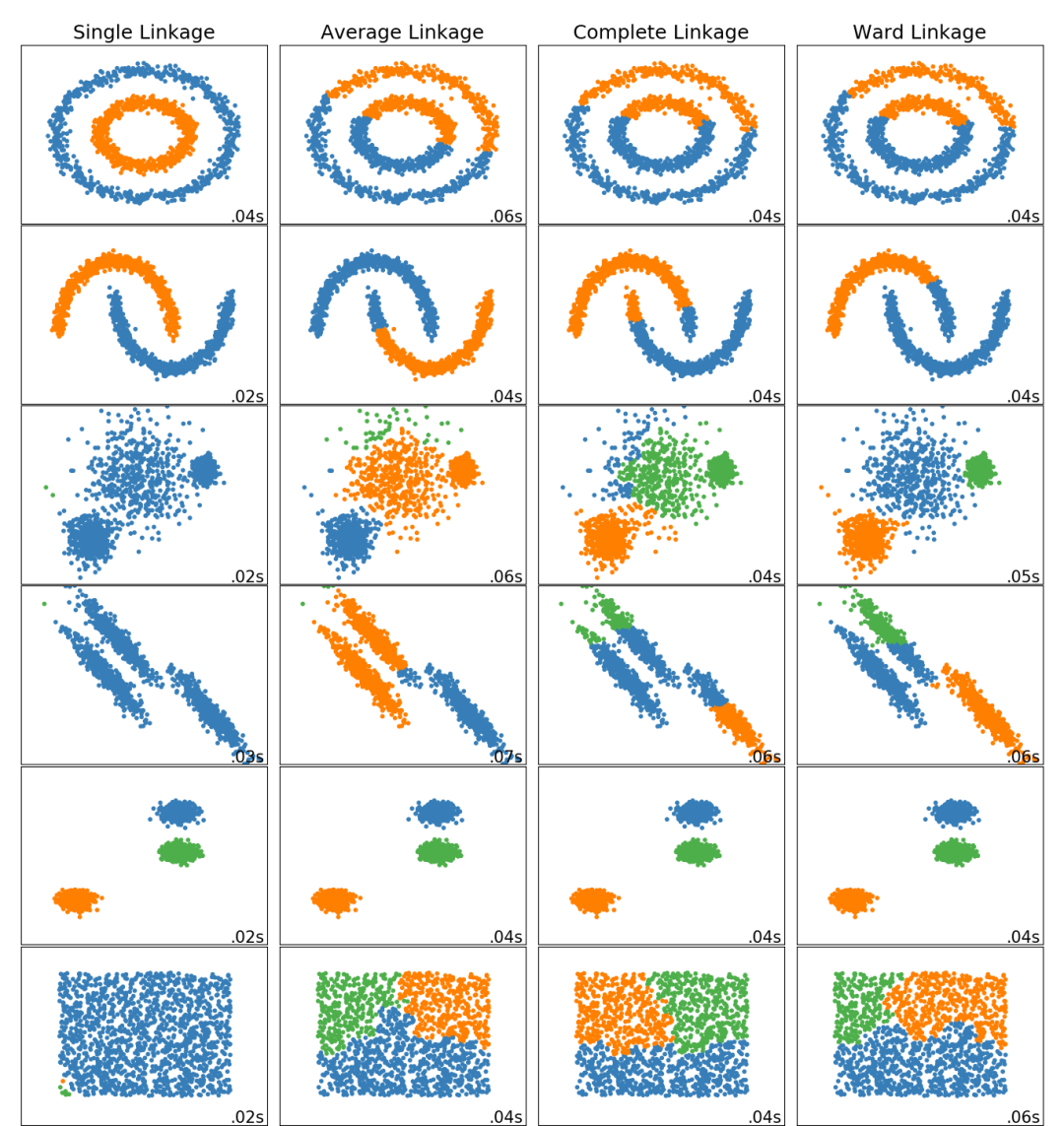

sphx_glr_plot_linkage_comparison_001

脚本的总运行时间：(0分钟2.983秒) 估计的内存使用量： 8 MB

下载Python源代码: plot_linkage_comparison.py 下载Jupyter notebook源代码: plot_linkage_comparison.ipynb 由Sphinx-Gallery生成的画廊 ‍

文壹由“伴编辑器”提供技术支持

☆☆☆为方便大家查阅，小编已将scikit-learn学习路线专栏 文章统一整理到公众号底部菜单栏，同步更新中，关注公众号，点击左下方“系列文章”，如图：

欢迎大家和我一起沿着scikit-learn文档这条路线，一起巩固机器学习算法基础。(添加微信：mthler，备注：sklearn学习，一起进【sklearn机器学习进步群】开启打怪升级的学习之旅。)