sklearn gridsearchcv_使用python+sklearn实现概率PCA和因子分析进行模型选择

概率PCA和因子分析都是概率模型，新数据的似然性(likelihood)可用于模型选择和协方差估计。在这里，我们将在均等噪声(每个特征的噪声方差相同)或异方差噪声(每个特征的噪声方差均不同)损坏的低秩(low rank)数据上进行交叉验证比较PCA和FA，然后我们将模型似然性与从收缩协方差估计器中获得的似然性进行比较。

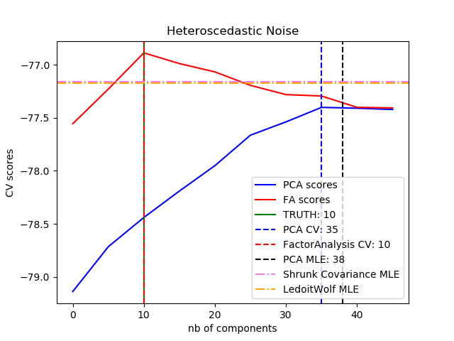
可以观察到，在均等噪声的情况下，FA和PCA都成功地恢复了低秩子空间的大小，但PCA的似然性高于FA；而当存在异方差噪声时，PCA会高估了秩(rank)。在适当情况下，低秩模型比收缩模型的性能更高。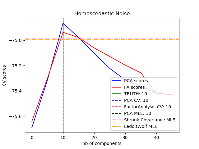

sphx_glr_plot_pca_vs_fa_model_selection_001

sphx_glr_plot_pca_vs_fa_model_selection_002

输出：

best n_components by PCA CV = 10
best n_components by FactorAnalysis CV = 10
best n_components by PCA MLE = 10
best n_components by PCA CV = 35
best n_components by FactorAnalysis CV = 10
best n_components by PCA MLE = 38

# 作者：Alexandre Gramfort#          Denis A. Engemann# 许可证：BSD 3 clauseimport numpy as npimport matplotlib.pyplot as pltfrom scipy import linalgfrom sklearn.decomposition import PCA, FactorAnalysisfrom sklearn.covariance import ShrunkCovariance, LedoitWolffrom sklearn.model_selection import cross_val_scorefrom sklearn.model_selection import GridSearchCV
print(__doc__)# ############################################################################## 创建数据
n_samples, n_features, rank = 1000, 50, 10
sigma = 1.
rng = np.random.RandomState(42)
U, _, _ = linalg.svd(rng.randn(n_features, n_features))
X = np.dot(rng.randn(n_samples, rank), U[:, :rank].T)# 添加均等噪声
X_homo = X + sigma * rng.randn(n_samples, n_features)# 添加异方差噪声
sigmas = sigma * rng.rand(n_features) + sigma / 2.
X_hetero = X + rng.randn(n_samples, n_features) * sigmas# ############################################################################## 拟合模型
n_components = np.arange(0, n_features, 5)  # options for n_componentsdef compute_scores(X):
    pca = PCA(svd_solver='full')
    fa = FactorAnalysis()
    pca_scores, fa_scores = [], []for n in n_components:
        pca.n_components = n
        fa.n_components = n
        pca_scores.append(np.mean(cross_val_score(pca, X)))
        fa_scores.append(np.mean(cross_val_score(fa, X)))return pca_scores, fa_scoresdef shrunk_cov_score(X):
    shrinkages = np.logspace(-2, 0, 30)
    cv = GridSearchCV(ShrunkCovariance(), {'shrinkage': shrinkages})return np.mean(cross_val_score(cv.fit(X).best_estimator_, X))def lw_score(X):return np.mean(cross_val_score(LedoitWolf(), X))for X, title in [(X_homo, 'Homoscedastic Noise'),
                 (X_hetero, 'Heteroscedastic Noise')]:
    pca_scores, fa_scores = compute_scores(X)
    n_components_pca = n_components[np.argmax(pca_scores)]
    n_components_fa = n_components[np.argmax(fa_scores)]
    pca = PCA(svd_solver='full', n_components='mle')
    pca.fit(X)
    n_components_pca_mle = pca.n_components_
    print("best n_components by PCA CV = %d" % n_components_pca)
    print("best n_components by FactorAnalysis CV = %d" % n_components_fa)
    print("best n_components by PCA MLE = %d" % n_components_pca_mle)
    plt.figure()
    plt.plot(n_components, pca_scores, 'b', label='PCA scores')
    plt.plot(n_components, fa_scores, 'r', label='FA scores')
    plt.axvline(rank, color='g', label='TRUTH: %d' % rank, linestyle='-')
    plt.axvline(n_components_pca, color='b',
                label='PCA CV: %d' % n_components_pca, linestyle='--')
    plt.axvline(n_components_fa, color='r',
                label='FactorAnalysis CV: %d' % n_components_fa,
                linestyle='--')
    plt.axvline(n_components_pca_mle, color='k',
                label='PCA MLE: %d' % n_components_pca_mle, linestyle='--')# 与其他协方差估计器进行比较
    plt.axhline(shrunk_cov_score(X), color='violet',
                label='Shrunk Covariance MLE', linestyle='-.')
    plt.axhline(lw_score(X), color='orange',
                label='LedoitWolf MLE' % n_components_pca_mle, linestyle='-.')
    plt.xlabel('nb of components')
    plt.ylabel('CV scores')
    plt.legend(loc='lower right')
    plt.title(title)
plt.show()

脚本的总运行时间：( 0 分 8.397 秒) 估计的内存使用量：8 MB

由Sphinx-Gallery生成的画廊

下载python源代码:plot_faces_decomposition.py

下载Jupyter notebook源代码:plot_faces_decomposition.ipynb

☆☆☆为方便大家查阅，小编已将scikit-learn学习路线专栏文章统一整理到公众号底部菜单栏，同步更新中，关注公众号，点击左下方“系列文章”，如图： 欢迎大家和我一起沿着scikit-learn文档这条路线，一起巩固机器学习算法基础。(添加微信：mthler，备注：sklearn学习，一起进【sklearn机器学习进步群】开启打怪升级的学习之旅。)

‍