tushare pro接口_alphalens+tushare 因子检验的快速实现

本文所有结论均来自网上数据，研究仅供学习讨论，请勿作为投资参考。

alphalens是著名的量化平台quantopian（国内许多量化平台的原型）开源的几大量化分析工具之一，提供了完整的因子分析流程。

tushare是Jimmy大神开发的国内财经数据接口包，推荐使用最近刚更新的pro版，接口更加清晰。

利用alphalens和tushare，能够快速实现A股的因子检验。

本次的教程基于python2.7

首先安装alphalens：

稳定版：

pip install alphalens

或者开发版：

pip install git+https://github.com/quantopian/alphalens

安装tushare：

pip install tushare

使用tushare pro首先得去官网注册： https://tushare.pro

注册好之后在个人主页获取token

设置token：

import pandas as pd 
import numpy as np
import tushare as ts
import alphalens 

ts.set_token('your token here')

获取交易日历：

pro = ts.pro_api()
wdays = pro.trade_cal(exchange_id='', start_date='20180101', end_date='20180831')
wdays = wdays[wdays.is_open==1].cal_date.values.tolist()

获取每天的因子数据（原文链接有数据可供直接下载）：

factors_list = []
for idate in wdays : 
    temp_df = pro.query('daily_basic', ts_code='', trade_date=idate)
    factors_list.append(temp_df)
factor_df = pd.concat(factors_list)

获取每支股票的前复权价格，为了提高效率，采取多进程下载（原文链接有数据可供直接下载）：

def worker(iticker):
    print(iticker)
    temp_quote = None
    try:
        ticker = iticker.split('.')[0]
        temp_quote = ts.get_k_data(ticker,start='2018-01-01',end='2018-08-31',autype = 'qfq').loc[:,['date','close']]
        temp_quote['ts_code'] = iticker
        return temp_quote
    except:
        return None

quote_list = []
tickers = list(set(factor_df.ts_code))

from multiprocessing import Pool
pool = Pool(8)
res = pool.map(worker,tickers)
quotes = pd.concat(res)
quotes.rename(columns={'date':'trade_date'},inplace=True)

对日期格式做处理：

factor_df.trade_date = pd.to_datetime(factor_df.trade_date.astype('str'))
quotes.trade_date = pd.to_datetime(quotes.trade_date)

目前tushare提供的因子数据包括三大表以及一些常见的财务指标（具体的数据接口参考文档），这里我们使用ps_ttm作为测试因子：

factor = factor_df.loc[:,['ts_code','trade_date','ps_ttm']].set_index(['trade_date','ts_code'])
factor = factor.unstack().fillna(method='ffill').stack()

reshape数据格式以满足alphalens的要求：

prices = quotes.pivot(index='trade_date',columns='ts_code',values='close')

因子收益率分析

有了因子和价格数据之后可以开始正式的因子分析， 通过alphalens.utils.get_clean_factor_and_forward_returns可以得到当日因子值， n period之后的股票收益率，以及因子的分位数区间：

factor_data = alphalens.utils.get_clean_factor_and_forward_returns(
    factor,
    prices,
    groupby=None,
    quantiles=5,
    periods=(10,20,40),
    filter_zscore=None)

groupby 是股票的分组信息，通常是股票的行业分类，这里我们不对每个行业做单独分析，因此取None。

quantiles 是将根据因子将股票分为几组，后续需要统计每组的收益率。

periods是研究因子有效日期的参数。

filter_zscore 是将超过n个标准差之外的因子值标准为nan。

计算mean return by quantile :

mean_return_by_q_daily, std_err = alphalens.performance.mean_return_by_quantile(factor_data, by_date=True)
mean_return_by_q, std_err_by_q = alphalens.performance.mean_return_by_quantile(factor_data, by_date=False)

其中mean_return_by_q_daily和mean_return_by_q分别代表每日的mean return 和 mean return统计值

每组收益的 bar plot 和 violin plot ：

alphalens.plotting.plot_quantile_returns_bar(mean_return_by_q)

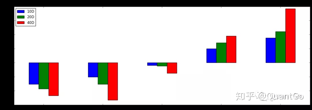
alphalens.plotting.plot_quantile_returns_violin(mean_return_by_q_daily)

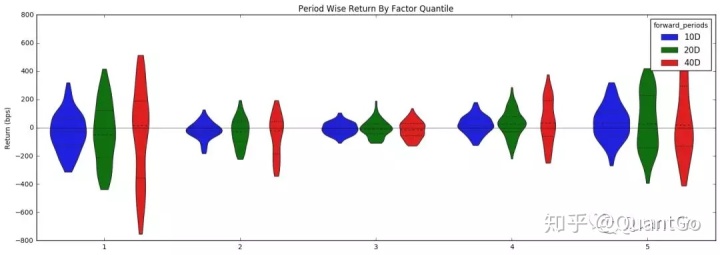
第五组存在明显的超额收益，说明ps是一个相对有效的因子

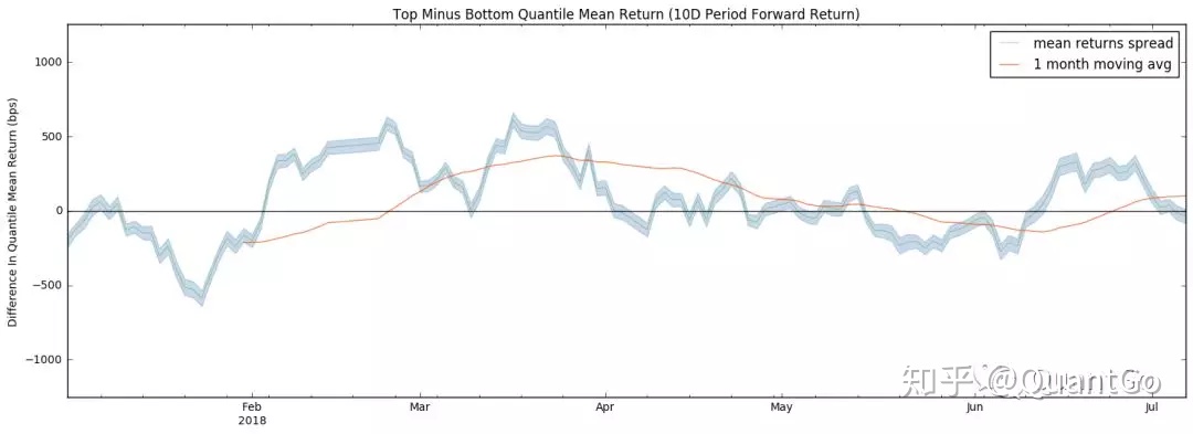
计算第一组和第五组的return 之差：

quant_return_spread, std_err_spread = alphalens.performance.compute_mean_returns_spread(mean_return_by_q_daily,
                                                                                        upper_quant=5,
                                                                                        lower_quant=1,
                                                                                        std_err=std_err)

画图：

alphalens.plotting.plot_mean_quantile_returns_spread_time_series(quant_return_spread, std_err_spread);

分组累计收益：

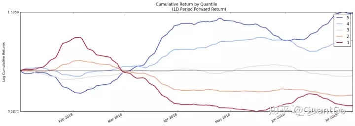
alphalens.tears.create_returns_tear_sheet(factor_data)

可以得到上述所有结果，不必一步一步运行

因子IC分析

除去分析因子的分组收益率，常见的因子分析方法是根据因子和收益率之间的相关性来分析因子，这种方法称为IC分析

From Wikipedia...

The information coefficient (IC) is a measure of the merit of a predicted value. In finance, the information coefficient is used as a performance metric for the predictive skill of a financial analyst. The information coefficient is similar to correlation in that it can be seen to measure the linear relationship between two random variables, e.g. predicted stock returns and the actualized returns. The information coefficient ranges from 0 to 1, with 0 denoting no linear relationship between predictions and actual values (poor forecasting skills) and 1 denoting a perfect linear relationship (good forecasting skills).

计算ic:

ic = alphalens.performance.factor_information_coefficient(factor_data)

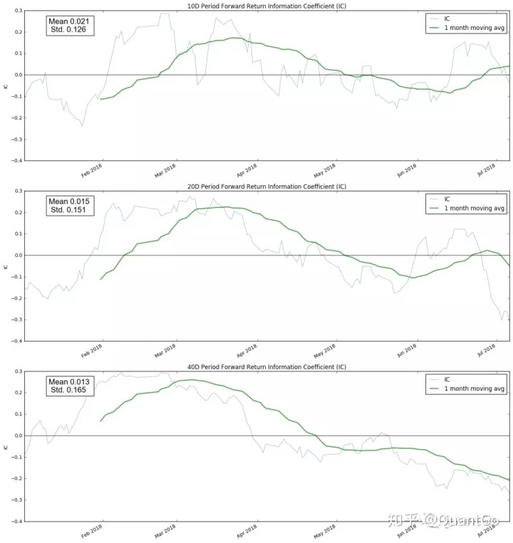
ic的时间序列：

alphalens.plotting.plot_ic_ts(ic)

ic 分布的 ：

alphalens.plotting.plot_ic_hist(ic);

ic的rolling 1m的均值：

mean_monthly_ic = alphalens.performance.mean_information_coefficient(factor_data, by_time='M')

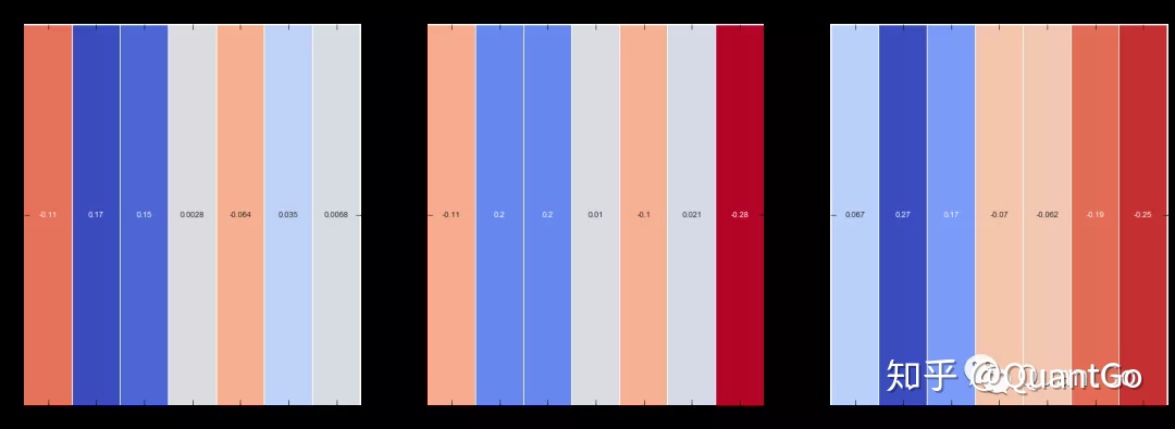
热力图：

alphalens.plotting.plot_monthly_ic_heatmap(mean_monthly_ic);

利用

alphalens.tears.create_information_tear_sheet(factor_data)

可以得到完整的ic分析结果

之后还有因子的turnonver分析，篇幅有限，就不再介绍。 因子分析只是alphalens的功能之一，还有event driven study等功能，总之是一款非常强大的工具。

后续我们还会介绍quantopian的其他package 以及一些其他的开源数据。