python读取can_Python 数据处理实例练习1：Pandas与数据可视化入门

数据收集、清洗、整理与数据可视化是Python数据处理的第一步，本练习通过一个实际的数据集(加拿大移民人口数据)，对Pandas，Matplotlib库进行基本讲解。主要的数据可视化在python下依赖matplotlib和pandas，如果已经安装了Anaconda发行版，则这两个库默认都已经安装，如果只是安装Jupyter Notebook，则可以直接通过命令行命令进行安装。

!pip install pandas!pip install matplotlib

1. 数据集引入

示例数据集来自加拿大官方移民数据，数据年限仅截止到2013年。首先，需要导入numpy和pandas两个库，对数据进行基本分析。因为数据是excel格式的(这是最广泛的数据格式之一，还需要安装xlrd库)，在Anaconda和标准Python发行版下通过下列两个命令可以分别实现安装。

!pip install xlrd!conda install -c anaconda xlrd --yes

需要注意的一点是，在Jupyter Notebook中安装包之后，内核可能不能马上导入使用，可以点击Kernel菜单下的Restart选项重新启动Kernel就可以恢复正常。

import numpy as np # useful for many scientific computing in Pythonimport pandas as pd # primary data structure library

读取示例数据并显示头/尾。

df_can = pd.read_excel('https://ibm.box.com/shared/static/lw190pt9zpy5bd1ptyg2aw15awomz9pu.xlsx', sheet_name='Canada by Citizenship', skiprows=range(20), skipfooter=2)print ('Data read into a pandas dataframe!')df_can.head()# tip: 如果需要显示更多行可以指定数据，比如 df_can.head(10) 

5 rows × 43 columns

df_can.tail()

5 rows × 43 columns

其他基本的查询指令，可以参考pandas的API文档。

df_can.info()df_can.columns.values df_can.index.valuesprint(type(df_can.columns))print(type(df_can.index))df_can.columns.tolist()df_can.index.tolist()print (type(df_can.columns.tolist()))print (type(df_can.index.tolist()))# size of dataframe (rows, columns)df_can.shape (195, 43)

数据清洗与整理

对数据集需要做一些基本的清洗与整理，下列几个步骤分别去掉不需要的列，对部分列重新命名使得更具有可读性，并增加了一个汇总列。

# in pandas axis=0 represents rows (default) and axis=1 represents columns.df_can.drop(['AREA','REG','DEV','Type','Coverage'], axis=1, inplace=True)df_can.head(2)

2 rows × 38 columns

df_can.rename(columns={'OdName':'Country', 'AreaName':'Continent', 'RegName':'Region'}, inplace=True)df_can.columnsIndex([ 'Country', 'Continent', 'Region', 'DevName', 1980, 1981, 1982, 1983, 1984, 1985, 1986, 1987, 1988, 1989, 1990, 1991, 1992, 1993, 1994, 1995, 1996, 1997, 1998, 1999, 2000, 2001, 2002, 2003, 2004, 2005, 2006, 2007, 2008, 2009, 2010, 2011, 2012, 2013], dtype='object')df_can['Total'] = df_can.sum(axis=1)df_can.isnull().sum()

2. Pandas中级功能，索引与选择

先看看当下的数据集信息，然后通过练习熟悉各种索引的使用方式。

df_can.describe()

8 rows × 35 columns

df_can.Country # 查找并返回所有国家列表df_can[['Country', 1980, 1981, 1982, 1983, 1984, 1985]] # 返回特定年份的值# 需要注意，国家名称是字符串类型而年份是整型# 为了保证格式统一，可以将所有名称均改为整型

195 rows × 7 columns

df_can.set_index('Country', inplace=True)# 将国家设置为索引项，与之相反的操作是 df_can.reset_index()df_can.head(3)

3 rows × 38 columns

# 也可以去掉索引项的名称df_can.index.name = None# 1. 显示日本籍移民(所有列)print(df_can.loc['Japan'])# 其他实现方式print(df_can.iloc[87])print(df_can[df_can.index == 'Japan'].T.squeeze())# 2. 2013年的数据print(df_can.loc['Japan', 2013])# 其他实现方式print(df_can.iloc[87, 36]) # 2013年是最后一列，总共36列982982# 3. 1980到1985年间的数据print(df_can.loc['Japan', [1980, 1981, 1982, 1983, 1984, 1984]])print(df_can.iloc[87, [3, 4, 5, 6, 7, 8]])1980 7011981 7561982 5981983 3091984 2461984 246Name: Japan, dtype: object1980 7011981 7561982 5981983 3091984 2461985 198Name: Japan, dtype: objectdf_can.columns = list(map(str, df_can.columns))# [print (type(x)) for x in df_can.columns.values] #

49 rows × 38 columns

# 可以通过多个条件进行筛选# l比如同时选择 AreaNAme = Asia 和RegName = Southern Asiadf_can[(df_can['Continent']=='Asia') & (df_can['Region']=='Southern Asia')]# 在使用逻辑操作符时， 需要用 '&' 和 '|' 取代 'and' 和 'or'# 不同条件需要分别通过括号分开。

9 rows × 38 columns

print ('data dimensions:', df_can.shape)print(df_can.columns)df_can.head(2)data dimensions: (195, 38)Index(['Continent', 'Region', 'DevName', '1980', '1981', '1982', '1983', '1984', '1985', '1986', '1987', '1988', '1989', '1990', '1991', '1992', '1993', '1994', '1995', '1996', '1997', '1998', '1999', '2000', '2001', '2002', '2003', '2004', '2005', '2006', '2007', '2008', '2009', '2010', '2011', '2012', '2013', 'Total'], dtype='object')

2 rows × 38 columns

3. 使用Matplotlib用以实现数据可视化

# %是Jupyter Notebook的魔术命令，这里使用inline即在文件中显示内容%matplotlib inline import matplotlib as mplimport matplotlib.pyplot as pltprint ('Matplotlib version: ', mpl.__version__) # >= 2.0.0 版本要大于2.0.0Matplotlib version: 3.0.2print(plt.style.available)mpl.style.use(['ggplot']) # optional: for ggplot-like style['bmh', 'classic', 'dark_background', 'fast', 'fivethirtyeight', 'ggplot', 'grayscale', 'seaborn-bright', 'seaborn-colorblind', 'seaborn-dark-palette', 'seaborn-dark', 'seaborn-darkgrid', 'seaborn-deep', 'seaborn-muted', 'seaborn-notebook', 'seaborn-paper', 'seaborn-pastel', 'seaborn-poster', 'seaborn-talk', 'seaborn-ticks', 'seaborn-white', 'seaborn-whitegrid', 'seaborn', 'Solarize_Light2', 'tableau-colorblind10', '_classic_test']haiti = df_can.loc['Haiti', years] # years参数见前节passing in years 1980 - 2013 to exclude the 'total' columnhaiti.head()1980 16661981 36921982 34981983 28601984 1418Name: Haiti, dtype: objecthaiti.plot()haiti.index = haiti.index.map(int) # 将海地的索引项改为整数以显示年份haiti.plot(kind='line')plt.title('Immigration from Haiti')plt.ylabel('Number of immigrants')plt.xlabel('Years')plt.show() # 本行用以显示图形

haiti.plot(kind='line')#可以在图形中添加标签plt.title('Immigration from Haiti')plt.ylabel('Number of Immigrants')plt.xlabel('Years')# 也可以在指定位置插入数据# syntax: plt.text(x, y, label)plt.text(2000, 6000, '2010 Earthquake') # see note belowplt.show()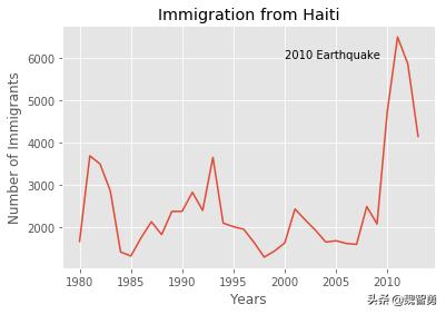 

以下程序用以显示中国和印度籍移民图示

df_CI=df_can.loc[['China','India'],years]df_CI.head()

1980198119821983198419851986198719881989…2004200520062007200820092010201120122013China5123668233081863152718161960264327584323…36619425843351827642300372962230391285023302434129India8880867081477338570442117150101891152210343…28235362103384828742282612945634235275093093333087

2 rows × 34 columns

df_CI.plot(kind='line')

上述的图形显然有问题，这主要是因为横轴纵轴错误，这是个常见的问题，需要通过transpose方法先修正。

df_CI = df_CI.transpose()df_CI.head()

ChinaIndia198051238880198166828670198233088147198318637338198415275704

df_CI.index = df_CI.index.map(int)df_CI.plot(kind='line')plt.title('Immigration from China and India')plt.ylabel('Number of Immigrants')plt.xlabel('Years')# annotate the 2010 Earthquake. # syntax: plt.text(x, y, label)plt.show()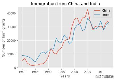 

df_can.sort_values(by='Total', ascending=False, axis=0, inplace=True)df_top5 = df_can.head(5)df_top5 = df_top5[years].transpose() print(df_top5) India China United Kingdom of Great Britain and Northern Ireland 1980 8880 5123 22045 1981 8670 6682 24796 1982 8147 3308 20620 1983 7338 1863 10015 1984 5704 1527 10170 1985 4211 1816 9564 1986 7150 1960 9470 1987 10189 2643 21337 1988 11522 2758 27359 1989 10343 4323 23795 1990 12041 8076 31668 1991 13734 14255 23380 1992 13673 10846 34123 1993 21496 9817 33720 1994 18620 13128 39231 1995 18489 14398 30145 1996 23859 19415 29322 1997 22268 20475 22965 1998 17241 21049 10367 1999 18974 30069 7045 2000 28572 35529 8840 2001 31223 36434 11728 2002 31889 31961 8046 2003 27155 36439 6797 2004 28235 36619 7533 2005 36210 42584 7258 2006 33848 33518 7140 2007 28742 27642 8216 2008 28261 30037 8979 2009 29456 29622 8876 2010 34235 30391 8724 2011 27509 28502 6204 2012 30933 33024 6195 2013 33087 34129 5827  Philippines Pakistan 1980 6051 978 1981 5921 972 1982 5249 1201 1983 4562 900 1984 3801 668 1985 3150 514 1986 4166 691 1987 7360 1072 1988 8639 1334 1989 11865 2261 1990 12509 2470 1991 12718 3079 1992 13670 4071 1993 20479 4777 1994 19532 4666 1995 15864 4994 1996 13692 9125 1997 11549 13073 1998 8735 9068 1999 9734 9979 2000 10763 15400 2001 13836 16708 2002 11707 15110 2003 12758 13205 2004 14004 13399 2005 18139 14314 2006 18400 13127 2007 19837 10124 2008 24887 8994 2009 28573 7217 2010 38617 6811 2011 36765 7468 2012 34315 11227 2013 29544 12603 df_top5.index = df_top5.index.map(int) # let's change the index values of df_top5 to type integer for plottingdf_top5.plot(kind='line', figsize=(14, 8)) # pass a tuple (x, y) sizeplt.title('Immigration Trend of Top 5 Countries')plt.ylabel('Number of Immigrants')plt.xlabel('Years')plt.show()