分类任务如何用逻辑回归实现_如何使用逻辑回归从头开始创建分类器

在本文中，我将简要描述如何使用逻辑回归从零开始创建分类器。在实践中，您可能会使用诸如scikit-learn或tensorflow之类的包来完成这项工作，但是理解基本的方程和算法对于机器学习非常有帮助。

本文中的所有代码使用Python，所以让我们导入所有需要Python库:

# Import packages%matplotlib inlineimport matplotlib as mplimport matplotlib.pyplot as pltimport numpy as np# General plot parametersmpl.rcParams['font.size'] = 18mpl.rcParams['axes.linewidth'] = 2mpl.rcParams['axes.spines.top'] = Falsempl.rcParams['axes.spines.right'] = Falsempl.rcParams['axes.labelpad'] = 10mpl.rcParams['xtick.major.size'] = 10mpl.rcParams['xtick.major.width'] = 2mpl.rcParams['ytick.major.size'] = 10mpl.rcParams['ytick.major.width'] = 2

离散预测

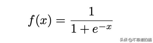
要理解预测算法，最好先选择一个数学函数，它的二进制输出是0或1。我们可以使用logistic或sigmoid函数，它的形式是:

我们可以用Python编写此函数并将其绘制如下：

def sigmoid(z):    """Returns value of the sigmoid function."""    return 1/(1 + np.exp(-z))# Calculate sigmoidx = np.linspace(-10, 10, 100)y = sigmoid(x)# Create figurefig = plt.figure(figsize=(8, 4))ax = fig.add_subplot(111)# Plot sigmoidax.plot(x, y, linewidth=2, color='#483d8b')# Add gridax.grid(linestyle='--', linewidth=2, color='gray', alpha=0.2)# Edit y-ticksax.set_yticks([0, 0.25, 0.5, 0.75, 1.0])# Edit axis labelsax.set(xlabel='x', ylabel='y')plt.show()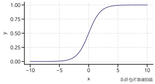

在x = 0附近，sigmoid函数的输出值迅速从0附近变为接近1。由于输出值在y = 0.5附近是对称的，我们可以将其作为决策阈值，其中y≥0.5输出1,y < 0.5输出0。

生成机器学习数据集

我们的场景如下所示：我们正在构建一个简单的电影推荐系统，该系统考虑到0到5之间的user score(所有用户)和0到5之间的critic score。然后，我们的模型应该根据输入数据生成一个决策边界，以预测当前用户是否会喜欢这部电影，并向他们推荐这部电影。

我们将为100部电影设置一组随机的user scores和critic scores：

# For reproducibility - will seed psuedorandom numbers at same pointnp.random.seed(74837)# Random user and critic scoresuser_score = 5*np.random.random(size=100)critic_score = 5*np.random.random(size=100)

现在，让我们生成分类：在这种情况下，用户可能喜欢这部电影(1)，也可能不喜欢(0)。为此，我们将使用以下决策边界函数。我们将此方程的右侧设置为0，因为它定义了logistic函数等于0.5的情况:

y = np.zeros(len(user_score))boundary = lambda x1, x2: 6 - x1 - 2*x2# Set y = 1 above decision boundaryfor i in range(len(y)):    if boundary(user_score[i], critic_score[i]) <= 0:        y[i] = 1    else:        y[i] = 0

注意，在实际数据集中，您不知道决策边界的函数形式是什么。在本教程中，我们定义了一个函数并添加了一些噪声。

现在，我们可以绘制我们的初始数据，其中一个橙色圆圈表示用户喜欢的电影，一个蓝色圆圈表示用户不喜欢的电影:

# Create figurefig = plt.figure(figsize=(6, 6))ax = fig.add_subplot(111)# Colors for scatter pointscolors = ['#483d8b', '#cc8400']colors_data = [colors[int(i)] for i in y]# Plot sample dataax.scatter(user_score, critic_score, color=colors_data, s=100, edgecolor='black', linewidth=2, alpha=0.7)# Add gridax.grid(linestyle='--', linewidth=2, color='gray', alpha=0.2)# Add axis labelsax.set(xlabel='User Score', ylabel='Critic Score')plt.show()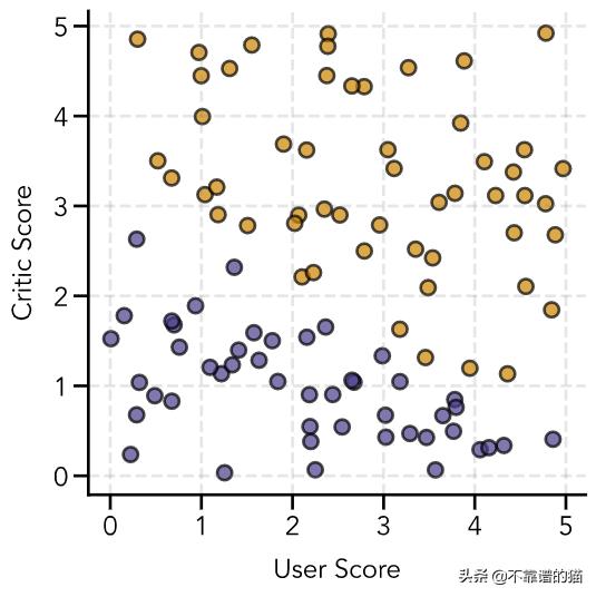

决策边界

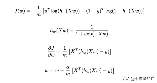
为了确定我们的决策边界有多好，我们需要为错误预测定义一个惩罚，我们将通过创建一个成本函数来实现。我们的预测如下:

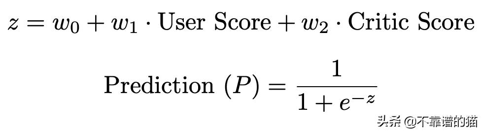
当P ≥0.5，我们输出1，当P <0.5，我们将输出0，其中W 0，W 1，W 2是需要优化的权重。

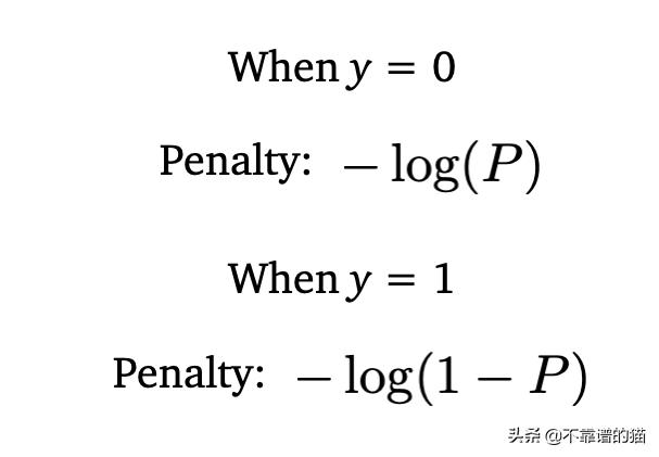
为了惩罚错误的分类，我们可以利用对数函数，因为log(1)= 0并且log(0)→-∞。我们可以使用它来创建两个惩罚(penalty)函数，如下所示：

我们可以将其可视化以更清楚地看到这些惩罚函数的效果：

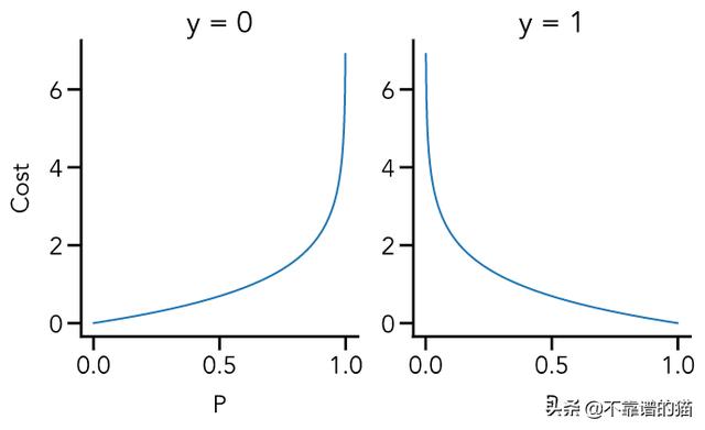
利用输出(y)不是0就是1的事实，我们可以将这两个惩罚(penalty)函数结合在一个表达式中，这个表达式包含了这两种情况:

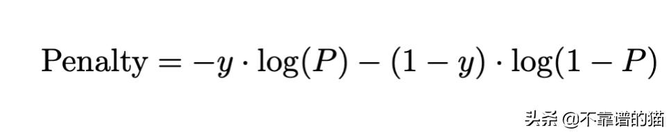
现在，当我们的输出是1，我们预测的结果接近于0(第一项)时，我们会遭受高惩罚。类似地，当我们的输出为0，我们预测的结果接近于1(第二项)时，也会发生相同的情况。

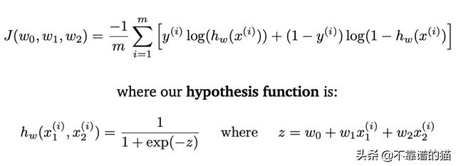
现在，我们可以采用惩罚函数并将其推广到m个训练实例中，第i个训练实例的标签由(i)表示。我们还将总成本除以m，以获得均值惩罚(就像线性回归中的均方误差一样)。该最终表达式也称为成本函数。我们将我们的两个特征(user score和critic score)称为x₁和x₂。

成本函数

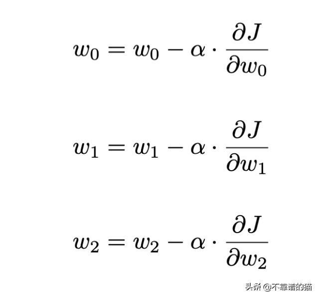
为了找到最佳决策边界，我们必须最小化成本函数，这可以通过梯度下降算法来完成，该算法的本质是：(1)通过计算成本函数的梯度来找到最大减少的方向，(2)通过沿着这个梯度移动来更新权重值。为了更新权重，我们还提供了学习率(α)，它确定了我们沿着该梯度移动了多少。选择学习率时需要权衡注意：学习率太小，我们的算法需要太长时间才能收敛；学习率太大，我们的算法实际上可能不会收敛到全局最优值。

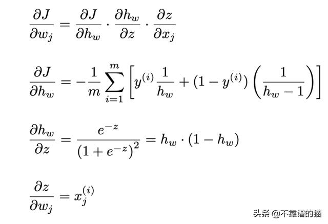
最后一个难题是计算上面表达式中的偏导数。我们可以用微积分的链式法则把它分解为:

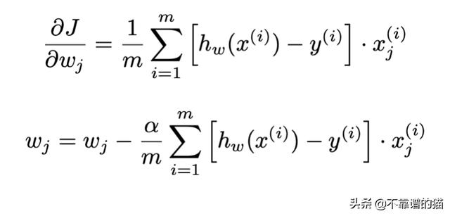
现在，我们可以把它们放在一起，得到以下梯度表达式和梯度下降更新规则:

初始化变量

首先，我们将变量初始化如下：

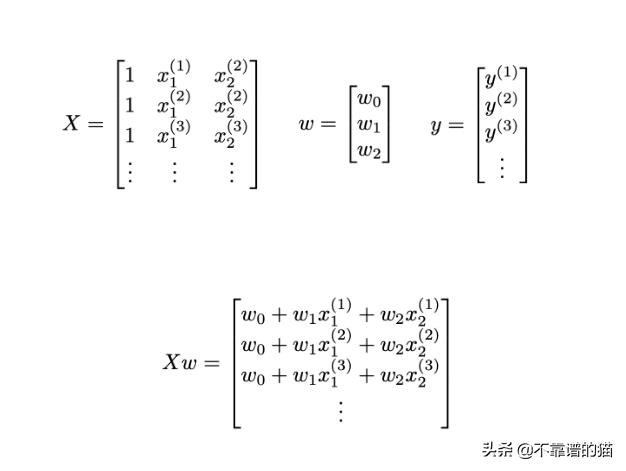
我们现在可以重写前面的函数下，其中上标T表示矩阵的转置:

我们的变量可以初始化如下(我们将所有权重设置为0):

X = np.concatenate((np.ones(shape=(len(user_score), 1)), user_score.reshape(len(user_score), 1),                     critic_score.reshape(len(critic_score), 1)), axis=1)y = y.reshape(len(y), 1)w = np.zeros(shape=(3, 1))

训练模型

以下函数计算成本和梯度值:

def cost_function(X, y, w):    """    Returns cost function and gradient    Parameters        X: m x (n+1) matrix of features        y: m x 1 vector of labels        w: (n+1) x 1 vector of weights    Returns        cost: value of cost function        grad: (n+1) x 1 vector of weight gradients    """        m = len(y)    h = sigmoid(np.dot(X, w))    cost = (1/m)*(-np.dot(y.T, np.log(h)) - np.dot((1 - y).T, np.log(1 - h)))    grad = (1/m)*np.dot(X.T, h - y)    return cost, grad

在定义梯度下降函数时，我们必须添加一个称为num_iter的额外输入，它告诉算法在返回最终优化权重之前要进行的迭代次数。

def gradient_descent(X, y, w, alpha, num_iters):    """    Uses gradient descent to minimize cost function.        Parameters        X: m x (n+1) matrix of features        y: m x 1 vector of labels        w: (n+1) x 1 vector of weights        alpha (float): learning rate        num_iters (int): number of iterations    Returns        J: 1 x num_iters vector of costs        w_new: (n+1) x 1 vector of optimized weights        w_hist: (n+1) x num_iters matrix of weights    """    w_new = np.copy(w)    w_hist = np.copy(w)    m = len(y)    J = np.zeros(num_iters)    for i in range(num_iters):        cost, grad = cost_function(X, y, w_new)        w_new = w_new - alpha*grad        w_hist = np.concatenate((w_hist, w_new), axis=1)        J[i] = cost    return J, w_new, w_hist

现在，使用以下Python代码训练我们的机器学习模型！

J, w_train, w_hist = gradient_descent(X, y, w, 0.5, 2000)

在实际情况中，为了交叉验证和测试模型，我们需要拆分训练数据，但是本教程主要用于演示，我们将使用所有的训练数据。

为了确保实际上每次迭代都在降低成本函数的值，可视化图像的Python代码如下：

# Create figurefig = plt.figure(figsize=(6, 4))ax = fig.add_subplot(111)# Plot costsax.plot(range(len(J)), J, linewidth=2)# Add axis labelsax.set(xlabel='Iterations', ylabel='J(w)')plt.show()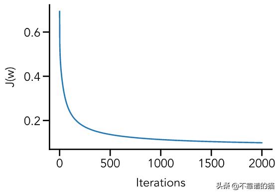

现在是关键时刻，我们可以绘制决策边界。我们将其覆盖到原始图上的方法是定义一个点网格，然后使用经过训练的权重计算sigmoid函数的预测值。

# Create figurefig = plt.figure(figsize=(6, 6))ax = fig.add_subplot(111)# Colors for scatter pointscolors = ['#483d8b', '#cc8400']colors_data = [colors[int(i)] for i in y]# Plot decision boundaryx1_bound, x2_bound = np.meshgrid(np.linspace(0, 5, 50), np.linspace(0, 5, 50))prob = sigmoid(w_train[0] + x1_bound*w_train[1] + x2_bound*w_train[2])ax.contour(x1_bound, x2_bound, prob, levels=[0.5], colors='black')# Plot sample dataax.scatter(user_score, critic_score, color=colors_data, s=100, edgecolor='black', linewidth=2, alpha=0.7)# Add gridax.grid(linestyle='--', linewidth=2, color='gray', alpha=0.2)# Add axis labelsax.set(xlabel='User Score', ylabel='Critic Score')plt.show()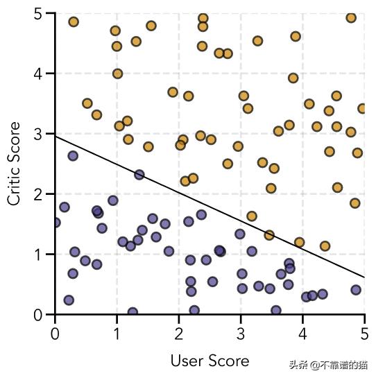

我们现在可以编写一个函数，根据这个训练好的模型做出预测:

def predict(X, w):    """    Predicts classifiers based on weights    Parameters        X: m x n matrix of features        w: n x 1 vector of weights        Returns        predictions: m x 1 vector of predictions    """    predictions = sigmoid(np.dot(X, w))    for i, val in enumerate(predictions):        if val >= 0.5:            predictions[i] = 1        else:            predictions[i] = 0    return predictions

现在，让我们对新实例进行预测：

X_new = np.asarray([[1, 3.4, 4.1], [1, 2.5, 1.7], [1, 4.8, 2.3]])print(predict(X_new, w_train))#[[1.] [0.]  [1.]]

多类分类

现在我们已经完成了制作二元分类器的所有工作，将其扩展到多类上是相当简单的。我们将使用一个名为one-vs-all的分类策略，其中我们为每个不同的类训练一个二元分类器，并选择sigmoid函数返回的最大值对应的类。

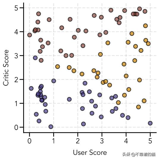
让我们构建模型：这次用户可以给电影评分0星，1星或2星。

首先，我们再次生成数据并应用两个决策边界：

np.random.seed(7839374)# Random user and critic scoresuser_score = 5*np.random.random(size=100)critic_score = 5*np.random.random(size=100)y = np.zeros(len(user_score))boundary_1 = lambda x1, x2: 6 - x1 - 2*x2boundary_2 = lambda x1, x2: 4 + x1 - 2*x2for i in range(len(y)):    if (boundary_1(user_score[i], critic_score[i]) + 0.5*np.random.normal() <= 0):        if (boundary_2(user_score[i], critic_score[i]) <= 0):            y[i] = 2        else:            y[i] = 1    else:        y[i] = 0# Create figurefig = plt.figure(figsize=(6, 6))ax = fig.add_subplot(111)# Colors for scatter pointscolors = ['#483d8b', '#cc8400', '#8b483d']colors_data = [colors[int(i)] for i in y]# Plot sample dataax.scatter(user_score, critic_score, color=colors_data, s=100, edgecolor='black', linewidth=2, alpha=0.7)# Add gridax.grid(linestyle='--', linewidth=2, color='gray', alpha=0.2)# Add axis labelsax.set(xlabel='User Score', ylabel='Critic Score')plt.show()

我们的数据集如下所示，其中蓝色圆圈代表0星，橙色圆圈代表1星，红色圆圈代表2星：

对于我们训练的每个二进制分类器，我们将需要重新标记数据，以便将我们感兴趣的类的输出设置为1，并将所有其他标签设置为0。例如，如果我们有3组A(0) ，B(1)和C(2)—我们必须制作三个二进制分类器：

对于我们训练的每个二元分类器，我们需要重新标记数据，以便我们感兴趣的类的输出被设置为1，其他标签被设置为0。我们必须创建3个二元分类器:

(1)A设为1，B和C设为0

(2)B设为1，A和C设为0

(3)C设为1，A和B设为0

下面的函数为每个分类器重新标记我们的数据:

def relabel_data(y, label):    """    Relabels data for one-vs-all classifier    Parameters        y: m x 1 vector of labels        label: which label to set to 1 (sets others to 0)        Returns        relabeled_data: m x 1 vector of relabeled data    """    relabeled_data = np.zeros(len(y))    for i, val in enumerate(y):        if val == label:            relabeled_data[i] = 1    return relabeled_data.reshape(len(y), 1)

现在，我们进行模型训练：

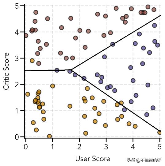
# Initialize variablesX = np.concatenate((np.ones(shape=(len(user_score), 1)), user_score.reshape(len(user_score), 1),                     critic_score.reshape(len(critic_score), 1)), axis=1)y = y.reshape(len(y), 1)w = np.zeros(shape=(3, 1))y_class1 = relabel_data(y, 0)_, w_class1, _ = gradient_descent(X, y_class1, w, 0.5, 2000)y_class2 = relabel_data(y, 1)_, w_class2, _ = gradient_descent(X, y_class2, w, 0.5, 2000)y_class3 = relabel_data(y, 2)_, w_class3, _ = gradient_descent(X, y_class3, w, 0.5, 2000)

绘制决策边界这一次稍微复杂一些。我们必须为每个经过训练的分类器计算网格中每个点的预测值。然后我们选择每个点的最大预测值，并根据导致该最大值的分类器为其分配相应的类。我们选择绘制的轮廓线为0.5(在0和1之间)和1.5(在1和2之间):

# Create figurefig = plt.figure(figsize=(6, 6))ax = fig.add_subplot(111)# Colors for scatter pointscolors = ['#cc8400', '#483d8b', '#8b483d']colors_data = [colors[int(i)] for i in y]# Plot decision boundariesx1_bound, x2_bound = np.meshgrid(np.linspace(-0.05, 5.05, 500), np.linspace(-0.05, 5.05, 500))prob_0 = sigmoid(w_class1[0] + x1_bound*w_class1[1] + x2_bound*w_class1[2])prob_1 = sigmoid(w_class2[0] + x1_bound*w_class2[1] + x2_bound*w_class2[2])prob_2 = sigmoid(w_class3[0] + x1_bound*w_class3[1] + x2_bound*w_class3[2])prob_max = np.zeros(shape=x1_bound.shape)for i in range(prob_max.shape[0]):    for j in range(prob_max.shape[1]):        maximum = max(prob_0[i][j], prob_1[i][j], prob_2[i][j])        if maximum == prob_0[i][j]:            prob_max[i][j] = 0        elif maximum == prob_1[i][j]:            prob_max[i][j] = 1        else:            prob_max[i][j] = 2ax.contour(x1_bound, x2_bound, prob_max, levels=[0.5, 1.5], colors='black', linewidths=2)# Plot sample dataax.scatter(user_score, critic_score, color=colors_data, s=100, edgecolor='black', linewidth=2, alpha=0.7)# Add gridax.grid(linestyle='--', linewidth=2, color='gray', alpha=0.2)# Add axis labelsax.set(xlim=(-0.05, 5.05), ylim=(-0.05, 5.05), xlabel='User Score', ylabel='Critic Score')plt.show()

这是我们训练过的决策边界！

最后，我们做一个预测函数。为此，我们将使用一个小技巧——我们将对每个实例中的每个分类器进行预测；接下来，我们将把每组预测作为一个新列附加到预测矩阵中；接下来通过遍历每一行并选择具有最大值的列索引，然后获得分类器标签！

def predict_multi(X, w):    """    Predicts classifiers based on weights    Parameters        X: m x n matrix of features        w: array of n x 1 vectors of weights        Returns        predictions: m x 1 vector of predictions    """    predictions = np.empty((X.shape[0], 0))    # Gather predictions for each classifier    for i in range(len(w)):        predictions = np.append(predictions, sigmoid(np.dot(X, w[i])), axis=1)    return np.argmax(predictions, axis=1).reshape(X.shape[0], 1)

X_new = np.array([[1, 1, 1], [1, 1, 4.2], [1, 4.5, 2.5]])print(predict_multi(X_new, [w_class1, w_class2, w_class3]))# [[0]      [2]       [1]]