机器学习ai选股_使用机器学习和AI的约会算法

在用户约会资料上使用无监督学习

> Photo by Alexander Sinn on Unsplash

约会对于单身人士来说是艰难的。 约会应用程序可能更粗糙。 约会应用程序使用的算法在很大程度上由使用它们的各个公司保密。 今天，我们将尝试通过使用AI和机器学习构建约会算法来阐明这些算法。 更具体地说，我们将以聚类的形式利用无监督的机器学习。

希望我们可以通过使用机器学习将用户配对来改善约会档案匹配的过程。 如果诸如Tinder或Hinge之类的约会公司已经利用了这些技术，那么我们至少将学到更多有关他们的个人资料匹配过程和一些无监督机器学习概念的知识。 但是，如果他们不使用机器学习，那么也许我们肯定可以自己改进配对过程。

在下面的上一篇文章中探讨并详细介绍了将机器学习用于约会应用程序和算法的想法。

应用机器学习找到爱情

开发AI Matchmaker的第一步

本文讨论了AI和约会应用程序的应用。 它列出了项目的大纲，我们将在本文中完成该大纲。 整体概念和应用很简单。 我们将使用K均值聚类或分层聚类聚类将约会资料相互聚类。 通过这样做，我们希望为这些假设的用户提供更多像他们自己的匹配，而不是像他们自己一样的个人资料。

现在我们有了一个大纲来开始创建这种机器学习约会算法，我们可以开始用Python对其进行编码！

获取约会资料数据

由于公开的约会配置文件很少或不可能获得，由于安全和隐私风险，这是可以理解的，因此我们将不得不使用伪造的约会配置文件来测试我们的机器学习算法。 以下文章概述了收集这些伪造的约会资料的过程：

生成数据科学的假约会资料

通过Web爬网伪造约会资料进行数据分析

拥有伪造的约会资料后，我们就可以开始使用自然语言处理(NLP)来探索和分析我们的数据(特别是用户履历)的实践。 我们还有另一篇文章详细介绍了整个过程：

在约会资料上使用NLP机器学习

为用户BIOS应用自然语言处理

通过收集和分析数据，我们将能够继续进行项目的下一个激动人心的部分-聚类！

准备配置文件数据

首先，我们必须首先导入所有必要的库，以使该聚类算法正常运行。 我们还将加载伪造的约会配置文件时创建的Pandas DataFrame。

# Librariesimport pandas as pdpd.set_option('display.max_colwidth', 500)import numpy as npimport matplotlib.pyplot as pltimport seaborn as snsimport _pickle as picklefrom sklearn.feature_extraction.text import TfidfVectorizer, CountVectorizerfrom sklearn.cluster import KMeans, AgglomerativeClusteringfrom sklearn.metrics import silhouette_score, davies_bouldin_scorefrom sklearn.preprocessing import MinMaxScaler# Loading in the cleaned DFwith open("profiles.pkl",'rb') as fp:    df = pickle.load(fp)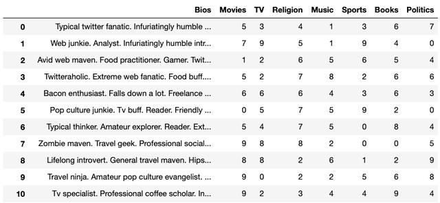

> The DataFrame containing all our data for each fake dating profile

有了良好的数据集，我们就可以开始进行聚类算法的下一步。

扩展数据

下一步将扩展约会类别(电影，电视，宗教等)，这将有助于我们的聚类算法的性能。 这将潜在地减少将聚类算法适合并将其转换为数据集所需的时间。

# Instantiating the Scalerscaler = MinMaxScaler()# Scaling the categories then replacing the old valuesdf = df[['Bios']].join( pd.DataFrame( scaler.fit_transform( df.drop('Bios',axis=1)), columns=df.columns[1:], index=df.index))

向量化BIOS

接下来，我们将必须对来自虚假配置文件的BIOS进行矢量化处理。 我们将创建一个包含矢量化的BIOS的新DataFrame，并删除原始的" Bio"列。 通过矢量化，我们将实现两种不同的方法，以查看它们是否对聚类算法产生重大影响。 这两种矢量化方法是：计数矢量化和TFIDF矢量化。 我们将尝试使用两种方法来找到最佳的矢量化方法。

# Instantiating the Vectorizer, experimenting with bothvectorizer = CountVectorizer()#vectorizer = TfidfVectorizer()# Fitting the vectorizer to the Biosx = vectorizer.fit_transform(df['Bios'])# Creating a new DF that contains the vectorized wordsdf_wrds = pd.DataFrame(x.toarray(), columns=vectorizer.get_feature_names())# Concating the words DF with the original DFnew_df = pd.concat([df, df_wrds], axis=1)# Dropping the Bios because it is no longer needed in place of vectorizationnew_df.drop('Bios', axis=1, inplace=True)

在这里，我们可以选择使用CountVectorizer()或TfidfVectorizer()对约会个人资料进行矢量化。 将Bios进行矢量化处理并放入其自己的DataFrame中后，我们会将它们与缩放的约会类别连接起来，以创建具有我们所需所有功能的新DataFrame。

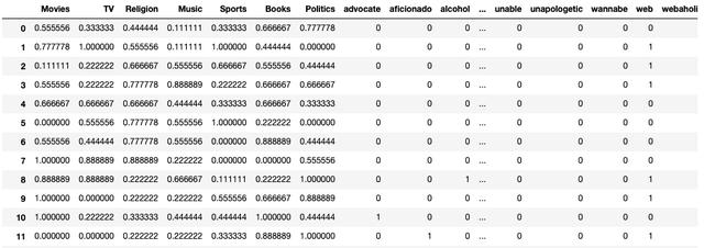
> Our DF that includes the vectorized bios and scaled dating categories

基于此最终DF，我们拥有100多个功能。 因此，我们将不得不使用主成分分析(PCA)来降低数据集的维数。

DataFrame上的PCA

为了减少大型功能集，我们将必须实施主成分分析(PCA)。 这种技术将减少我们数据集的维数，但仍保留许多可变性或有价值的统计信息。

# Importing the libraryfrom sklearn.decomposition import PCA# Instantiating PCApca = PCA()# Fitting and Transforming the DFdf_pca = pca.fit_transform(new_df)# Plotting to determine how many features should the dataset be reduced toplt.style.use("bmh")plt.figure(figsize=(14,4))plt.plot(range(1,new_df.shape[1]+1), pca.explained_variance_ratio_.cumsum())plt.show()# Finding the exact number of features that explain at least 95% of the variance in the datasettotal_explained_variance = pca.explained_variance_ratio_.cumsum()n_over_95 = len(total_explained_variance[total_explained_variance>=.95])n_to_reach_95 = new_df.shape[1] - n_over_95# Printing out the number of features needed to retain 95% varianceprint(f"Number features: {n_to_reach_95}Total Variance Explained: {total_explained_variance[n_to_reach_95]}")# Reducing the dataset to the number of features determined beforepca = PCA(n_components=n_to_reach_95)# Fitting and transforming the dataset to the stated number of features and creating a new DFdf_pca = pca.fit_transform(new_df)# Seeing the variance ratio that still remains after the dataset has been reducedprint(pca.explained_variance_ratio_.cumsum()[-1])

我们在这里所做的是拟合并变换我们的最后一个DF，然后绘制方差和特征数量。 该图将直观地告诉我们有多少个要素说明了差异。

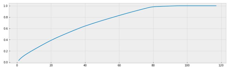
> # of Features accounting for % of the Variance

运行我们的代码后，构成差异95％的特征数量为74。牢记这一数字，我们可以将其应用于PCA函数，以将上一个DF中的主要组件或特征数量从减少到74。 117.现在，将使用这些功能代替原始DF来适应我们的聚类算法。

聚类约会概况

利用我们的数据缩放，矢量化和PCA，我们可以开始对约会资料进行聚类。 为了将配置文件聚类在一起，我们必须首先找到要创建的最佳聚类数。

聚类的评估指标

将根据特定的评估指标确定最佳的群集数量，这些评估指标将量化群集算法的性能。 由于没有要创建的确定数量的集群，因此我们将使用几个不同的评估指标来确定最佳集群数。 这些度量标准是"轮廓系数"和" Davies-Bouldin得分"。

这些指标各有其优点和缺点。 选择使用任一个都是纯粹主观的，如果您选择，则可以自由使用另一个指标。

找到正确数量的集群

下面，我们将运行一些代码，这些代码将使用不同数量的集群来运行集群算法。

# Setting the amount of clusters to test outcluster_cnt = [i for i in range(2, 20, 1)]# Establishing empty lists to store the scores for the evaluation metricss_scores = []db_scores = []# Looping through different iterations for the number of clustersfor i in cluster_cnt:        # Hierarchical Agglomerative Clustering with different number of clusters    hac = AgglomerativeClustering(n_clusters=i)        hac.fit(df_pca)        cluster_assignments = hac.labels_        ## KMeans Clustering with different number of clusters    #k_means = KMeans(n_clusters=i)        #k_means.fit(df_pca)        #cluster_assignments = k_means.predict(df_pca)        # Appending the scores to the empty lists        s_scores.append(silhouette_score(df_pca, cluster_assignments))        db_scores.append(davies_bouldin_score(df_pca, cluster_assignments))

通过运行此代码，我们将经历几个步骤：

· 为我们的聚类算法遍历不同数量的聚类。

· 使算法适合我们的PCA的DataFrame。

· 将配置文件分配给它们的集群。

· 将各个评估分数添加到列表中。 稍后将使用此列表来确定最佳群集数。

另外，还有一个选项可以在循环中运行两种类型的聚类算法：层次性聚类聚类和KMeans聚类。 有一个选项可以取消注释所需的聚类算法。

评估集群

为了评估聚类算法，我们将创建一个评估函数以在分数列表上运行。

def plot_evaluation(y, x=cluster_cnt):    """    Plots the scores of a set evaluation metric. Prints out the max and min values of the evaluation scores.    """        # Creating a DataFrame for returning the max and min scores for each cluster    df = pd.DataFrame(columns=['Cluster Score'], index=[i for i in range(2, len(y)+2)])    df['Cluster Score'] = y        print('Max Value:Cluster #', df[df['Cluster Score']==df['Cluster Score'].max()])    print('Min Value:Cluster #', df[df['Cluster Score']==df['Cluster Score'].min()])        # Plotting out the scores based on cluster count    plt.figure(figsize=(16,6))    plt.style.use('ggplot')    plt.plot(x,y)    plt.xlabel('# of Clusters')    plt.ylabel('Score')    plt.show()    # Running the function on the list of scoresplot_evaluation(s_scores)plot_evaluation(db_scores)

使用此功能，我们可以评估获得的分数列表，并绘制出值以确定最佳聚类数。

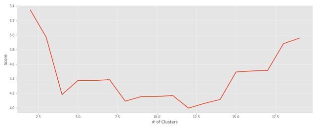
> Davies-Bouldin Score

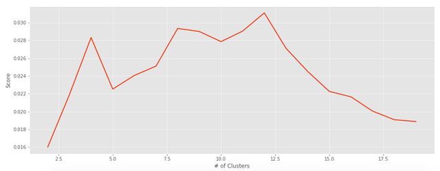
> Silhouette Coefficient Score

根据这些图表和评估指标，聚类的最佳数量似乎为12。对于我们的算法最后运行，我们将使用：

· 使用CountVectorizer来矢量化BIOS，而不是TfidfVectorizer。

· 分层聚集聚类而不是K表示聚类。

· 12个集群

使用这些参数或函数，我们将对约会配置文件进行聚类，并为每个配置文件分配一个数字，以确定它们属于哪个聚类。

运行最终聚类算法

一切准备就绪后，我们终于可以发现每个约会配置文件的聚类分配。

# Instantiating HAChac = AgglomerativeClustering(n_clusters=12)# Fittinghac.fit(df_pca)# Getting cluster assignmentscluster_assignments = hac.labels_# Unscaling the categories then replacing the scaled valuesdf = df[['Bios']].join(pd.DataFrame(scaler.inverse_transform(df.drop('Bios', axis=1)), columns=df.columns[1:], index=df.index))# Assigning the clusters to each profiledf['Cluster #'] = cluster_assignments# Viewing the dating profiles with cluster assignmentsdf

运行代码后，我们可以创建一个包含集群分配的新列。 现在，此新的DataFrame显示每个约会配置文件的分配。

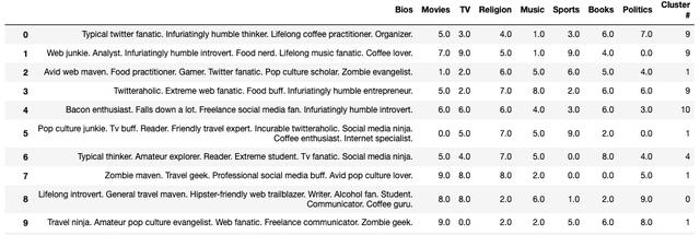
我们已经成功地将约会资料归类！ 现在，我们可以通过仅选择特定的集群编号来过滤DataFrame中的选择。 也许可以做更多的事情，但为简单起见，此聚类算法运作良好。

总结思想

通过利用无监督机器学习技术(例如，层次性聚类聚类)，我们成功地将5,000多个不同的约会配置文件聚在一起。 随时进行更改并尝试使用代码，以查看是否有可能改善总体结果。 希望到本文结尾，您能够了解有关NLP和无监督机器学习的更多信息。

此项目还有其他潜在的改进，例如实现一种方法来包括新的用户输入数据，以查看他们可能与谁匹配或聚类。 也许创建一个仪表板以完全实现该聚类算法作为原型约会应用程序。 总是有新颖而激动人心的方法可以从此处继续进行此项目，也许最终，我们可以通过该项目帮助解决人们的约会困扰。

(本文翻译自Marco Santos的文章《Dating Algorithms using Machine Learning and AI》，参考：https://towardsdatascience.com/dating-algorithms-using-machine-learning-and-ai-814b68ecd75e)