RNN的前世今生

什么是RNN？

RNN，即循环神经网络（Recurrent Neural Network），是一类以序列数据为输入，在序列的演进方向进行递归（recursion）且所有节点（循环单元）按链式连接的递归神经网络（recursive neural network）。

import tensorflow as tf
from tensorflow.examples.tutorials.mnist import input_data

tf.set_random_seed(1)

mnist = input_data.read_data_sets('MNIST_data', one_hot=True)

lr = 0.001
training_iters = 100000
batch_size = 128

n_inputs = 28   
n_steps = 28   
n_hidden_units = 128   
n_classes = 10      

x = tf.placeholder(tf.float32, [None, n_steps, n_inputs])
y = tf.placeholder(tf.float32, [None, n_classes])

weights = {

    'in': tf.Variable(tf.random_normal([n_inputs, n_hidden_units])),

    'out': tf.Variable(tf.random_normal([n_hidden_units, n_classes]))
}
biases = {

    'in': tf.Variable(tf.constant(0.1, shape=[n_hidden_units, ])),
   
    'out': tf.Variable(tf.constant(0.1, shape=[n_classes, ]))
}


def RNN(X, weights, biases):

    X = tf.reshape(X, [-1, n_inputs])
    X_in = tf.matmul(X, weights['in']) + biases['in']
    X_in = tf.reshape(X_in, [-1, n_steps, n_hidden_units])

    if int((tf.__version__).split('.')[1]) < 12 and int((tf.__version__).split('.')[0]) < 1:
        cell = tf.nn.rnn_cell.BasicLSTMCell(n_hidden_units, forget_bias=1.0, state_is_tuple=True)
    else:
        cell = tf.contrib.rnn.BasicLSTMCell(n_hidden_units)
   
    init_state = cell.zero_state(batch_size, dtype=tf.float32)
    outputs, final_state = tf.nn.dynamic_rnn(cell, X_in, initial_state=init_state, time_major=False)

    if int((tf.__version__).split('.')[1]) < 12 and int((tf.__version__).split('.')[0]) < 1:
        outputs = tf.unpack(tf.transpose(outputs, [1, 0, 2]))   
    else:
        outputs = tf.unstack(tf.transpose(outputs, [1,0,2]))
    results = tf.matmul(outputs[-1], weights['out']) + biases['out']    

    return results

pred = RNN(x, weights, biases)
cost = tf.reduce_mean(tf.nn.softmax_cross_entropy_with_logits(logits=pred, labels=y))
train_op = tf.train.AdamOptimizer(lr).minimize(cost)

correct_pred = tf.equal(tf.argmax(pred, 1), tf.argmax(y, 1))
accuracy = tf.reduce_mean(tf.cast(correct_pred, tf.float32))

with tf.Session() as sess:
   
    if int((tf.__version__).split('.')[1]) < 12 and int((tf.__version__).split('.')[0]) < 1:
        init = tf.initialize_all_variables()
    else:
        init = tf.global_variables_initializer()
    sess.run(init)
    step = 0
    while step * batch_size < training_iters:
        batch_xs, batch_ys = mnist.train.next_batch(batch_size)
        batch_xs = batch_xs.reshape([batch_size, n_steps, n_inputs])
        sess.run([train_op], feed_dict={
            x: batch_xs,
            y: batch_ys,
        })
        if step % 20 == 0:
            print(sess.run(accuracy, feed_dict={
            x: batch_xs,
            y: batch_ys,
            }))
        step += 1

RNN与CNN的区别

大家也许会有疑问，为什么有了CNN，还会有RNN呢？因为在CNN中，它的输入以及输出是相互独立的，比如图片分类的人、猫、狗这些标签都是分开的。

然而RNN中输入的却是序列，它的内容是相关的，也就是输出会依赖之前的输入序列，表达为当前时刻的输出是通过上一时刻的记忆和当前时刻共同决定的。也就是拥有记忆功能，对每个输入保留一些重要的信息。那么理论上最后就能得到整个输入的所有重要信息，进而综合考虑所有输入去预测输出。

之后在中间过程中，RNN中就通过激活函数将得到的信息进行过滤，大概可以理解为只保留、记住重要的信息。这个时候就可以tanh，去对一些不重要的信息进行过滤。当经过一层又一层的过滤后，就可以得到RNN的输出。这里我们使用的是softmax函数，通过softmax来预测出最大概率的输出。

小结

CNN的主要应用是图片的特征提取、识别、分类；而RNN的主要应用是文本生成、情感分析、机器翻译等。

双向RNN

在双向RNN中，假设当前t的输出不仅仅和之前的序列有关，并且还与之后的序列有关。那么，双向RNN通过增加从后往前传递信息的隐藏层来更灵活地处理这类信息。例如：预测一个语句中缺失的词语那么需要根据上下文进行预测；双向RNN是一个相对简单的RNN变形，由两个RNN上下叠加在一起组成，它的输出由这两个RNN的隐藏层的状态决定。

import tensorflow as tf
import numpy as np

from tensorflow.examples.tutorials.mnist import input_data
mnist = input_data.read_data_sets("/data/", one_hot=True)

learning_rate = 0.01
max_samples = 400000
batch_size = 128
display_step = 10

n_input = 28 
n_steps = 28
n_hidden = 256 
n_classes = 10 

x = tf.placeholder("float", [None, n_steps, n_input])
y = tf.placeholder("float", [None, n_classes])

weights = {
    'out': tf.Variable(tf.random_normal([2*n_hidden, n_classes]))
}
biases = {
    'out': tf.Variable(tf.random_normal([n_classes]))
}

def BiRNN(x, weights, biases):

    x = tf.transpose(x, [1, 0, 2])
    x = tf.reshape(x, [-1, n_input])
    x = tf.split(x, n_steps)

    lstm_fw_cell = tf.contrib.rnn.BasicLSTMCell(n_hidden, forget_bias=1.0)
    lstm_bw_cell = tf.contrib.rnn.BasicLSTMCell(n_hidden, forget_bias=1.0)

    outputs, _, _ = tf.contrib.rnn.static_bidirectional_rnn(lstm_fw_cell, lstm_bw_cell, x,dtype=tf.float32)

    return tf.matmul(outputs[-1], weights['out']) + biases['out']
    
pred = BiRNN(x, weights, biases)

cost = tf.reduce_mean(tf.nn.softmax_cross_entropy_with_logits(logits=pred, labels=y))
optimizer = tf.train.AdamOptimizer(learning_rate=learning_rate).minimize(cost)

correct_pred = tf.equal(tf.argmax(pred,1), tf.argmax(y,1))
accuracy = tf.reduce_mean(tf.cast(correct_pred, tf.float32))

init = tf.global_variables_initializer()

with tf.Session() as sess:
    sess.run(init)
    step = 1
    
    while step * batch_size < max_samples:
        batch_x, batch_y = mnist.train.next_batch(batch_size)
       
        batch_x = batch_x.reshape((batch_size, n_steps, n_input))
       
        sess.run(optimizer, feed_dict={x: batch_x, y: batch_y})
        if step % display_step == 0:
           
            acc = sess.run(accuracy, feed_dict={x: batch_x, y: batch_y})
           
            loss = sess.run(cost, feed_dict={x: batch_x, y: batch_y})
            print("Iter " + str(step*batch_size) + ", Minibatch Loss= " + \
                  "{:.6f}".format(loss) + ", Training Accuracy= " + \
                  "{:.5f}".format(acc))
        step += 1
    print("Optimization Finished!")

    test_len = 10000
    test_data = mnist.test.images[:test_len].reshape((-1, n_steps, n_input))
    test_label = mnist.test.labels[:test_len]
    print("Testing Accuracy:", \
        sess.run(accuracy, feed_dict={x: test_data, y: test_label}))

RNN注意事项

由于RNN特有的memory会影响后期其他的RNN的特点，梯度时大时小，学习率没法个性化的调整，导致RNN在train的过程中，Loss会震荡起伏，为了解决RNN的这个问题，在训练的时候，可以设置临界值，当梯度大于某个临界值，直接截断，用这个临界值作为梯度的大小，防止大幅震荡。

RNN之后的改良：GRU

由于上述所提及的，因为RNN中捕捉序列受步长距离设置影响的原因，其loss会震荡起伏，因此可能造成梯度爆炸或者梯度消失。之后就提出了新的网络，GRU，门控循环神经⽹络（gated recurrent neural network），它可以通过门的学习来控制序列中信息的流动，也因如此，可以解决捕捉时间序列中时间步距离较⼤的依赖关系。

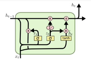
GRU的控制单位

在GRU中，有两种控制单位：重置⻔（reset gate）和更新⻔（update gate），通过，这些控制单位，可以修改循环神经⽹络中隐藏状态的计算⽅式。
在GRU中的重置⻔和更新⻔的输⼊均为当前时间步输⼊与上⼀时间步隐藏状态，输出由激活函数为sigmoid函数的全连接层计算得到。 sigmoid函数可以将元素的值变换到0和1之间。因此，重置⻔和更新⻔中每个元素的值域都是[0，1]。

• 重置⻔有助于捕捉时间序列⾥短期的依赖关系
• 更新⻔有助于捕捉时间序列⾥⻓期的依赖关系

候选隐藏状态

接下来，GRU的控制单元将计算候选隐藏状态来辅助稍后的隐藏状态计算。
如果重置⻔中元素值接近0，那么意味着重置对应隐藏状态元素为0，即丢弃上⼀时间步的隐藏状态。如果元素值接近1，那么表⽰保留上⼀时间步的隐藏状态。然后，将按元素乘法的结果与当前时间步的输⼊连结，再通过含激活函数tanh的全连接层计算出候选隐藏状态，其所有元素的值域为[-1,1]。

也就是说，重置⻔控制了上⼀时间步的隐藏状态如何流⼊当前时间步的候选隐藏状态。而上⼀时间步的隐藏状态可能包含了时间序列截⾄上⼀时间步的全部历史信息。因此，重置⻔可以⽤来丢弃与预测⽆关的历史信息。

隐藏状态

最后，当下时间t1的隐藏状态的计算通过使⽤当下时间t1的更新⻔来对上⼀时间步t2的隐藏状态和当下时间t1的候选隐藏状态做组合。
在这里，更新⻔可以控制隐藏状态应该如何被包含当前时间步信息的候选隐藏状态所更新。

GRU的优势

假设更新⻔在时间步之间⼀直近似1。那么，在时间步间的输⼊信息⼏乎没有流⼊时间步 t 的隐藏状态。 实际上，这可以看作是较早时刻的隐藏状态直通过时间保存并传递⾄当前时间步 t。
这个设计可以应对循环神经⽹络中的梯度衰减问题，并更好地捕捉时间序列中时间步距离较⼤的依赖关系。

LSTM

LSTM，也叫做⻓短期记忆（long short-term memory，LSTM）。它⽐⻔控循环单元的结构稍微复杂⼀点，也是为了解决在RNN网络中梯度衰减的问题，是GRU的一种扩展。
LSTM 中引⼊了3个⻔，即输⼊⻔（input gate）、遗忘⻔（forget gate）和输出⻔（output gate），以及与隐藏状态形状相同的记忆细胞（某些⽂献把记忆细胞当成⼀种特殊的隐藏状态），从而记录额外的信息。

LSTM在结构上，与GRU很类似：

1. 新的记忆都是根据之前状态及输入进行计算，但是GRU中有一个重置门控制之前状态的进入量，而在LSTM里没有类似门；
2. 产生新的状态方式不同，LSTM有两个不同的门，分别是遗忘门和输出门，而GRU只有一种更新门； LSTM对新产生的状态可以通过输出门进行调节，而GRU对输出无任何调节。
3. GRU的优点是这是个更加简单的模型，所以更容易创建一个更大的网络，而且它只有两个门，在计算性上也运行得更快，然后它可以扩大模型的规模。
4. LSTM更加强大和灵活，因为它有三个门而不是两个。

候选记忆细胞与记忆细胞

候选记忆细胞类似于网络中的隐藏层，只是当中使⽤了值域在[−1, 1]的tanh函数作为激活函数。
遗忘⻔控制上⼀时间步的记忆细胞中的信息是否传递到当前时间步，而输⼊⻔则控制当前时间步的输⼊通过候选记忆细胞如何流⼊当前时间步的记忆细胞。如果遗忘⻔⼀直近似且输⼊⻔⼀直近似0，过去的记忆细胞将⼀直通过时间保存并传递⾄当前时间步。这个设计可以应对循环神经⽹络中的梯度衰减问题，并更好地捕捉时间序列中时间步距离较⼤的依赖关系。

LSTM可以使用别的激活函数吗？

关于激活函数的选取，在LSTM中，遗忘门、输入门和输出门使用Sigmoid函数作为激活函数；在生成候选记忆时，使用双曲正切函数Tanh作为激活函数。值得注意的是，这两个激活函数都是饱和的，也就是说在输入达到一定值的情况下，输出就不会发生明显变化了。如果是用非饱和的激活函数，例如ReLU，那么将难以实现门控的效果。Sigmoid函数的输出在0～1之间，符合门控的物理定义。且当输入较大或较小时，其输出会非常接近1或0，从而保证该门开或关。在生成候选记忆时，使用Tanh函数，是因为其输出在−1～1之间，这与大多数场景下特征分布是0中心的吻合。此外，Tanh函数在输入为0附近相比Sigmoid函数有更大的梯度，通常使模型收敛更快。
当然，激活函数的选择也不是一成不变的，但要选择合理的激活函数。

import tensorflow as tf
import numpy as np
import matplotlib.pyplot as plt

BATCH_START = 0
TIME_STEPS = 20
BATCH_SIZE = 50
INPUT_SIZE = 1
OUTPUT_SIZE = 1
CELL_SIZE = 10
LR = 0.006

def get_batch():
    global BATCH_START, TIME_STEPS
    
    xs = np.arange(BATCH_START, BATCH_START+TIME_STEPS*BATCH_SIZE).reshape((BATCH_SIZE, TIME_STEPS)) / (10*np.pi)
    seq = np.sin(xs)
    res = np.cos(xs)
    BATCH_START += TIME_STEPS
    return [seq[:, :, np.newaxis], res[:, :, np.newaxis], xs]


class LSTMRNN(object):
    def __init__(self, n_steps, input_size, output_size, cell_size, batch_size):
        self.n_steps = n_steps
        self.input_size = input_size
        self.output_size = output_size
        self.cell_size = cell_size
        self.batch_size = batch_size
        with tf.name_scope('inputs'):
            self.xs = tf.placeholder(tf.float32, [None, n_steps, input_size], name='xs')
            self.ys = tf.placeholder(tf.float32, [None, n_steps, output_size], name='ys')
        with tf.variable_scope('in_hidden'):
            self.add_input_layer()
        with tf.variable_scope('LSTM_cell'):
            self.add_cell()
        with tf.variable_scope('out_hidden'):
            self.add_output_layer()
        with tf.name_scope('cost'):
            self.compute_cost()
        with tf.name_scope('train'):
            self.train_op = tf.train.AdamOptimizer(LR).minimize(self.cost)

    def add_input_layer(self,):
        l_in_x = tf.reshape(self.xs, [-1, self.input_size], name='2_2D')  
        
        Ws_in = self._weight_variable([self.input_size, self.cell_size])
        
        bs_in = self._bias_variable([self.cell_size,])
        
        with tf.name_scope('Wx_plus_b'):
            l_in_y = tf.matmul(l_in_x, Ws_in) + bs_in
        
        self.l_in_y = tf.reshape(l_in_y, [-1, self.n_steps, self.cell_size], name='2_3D')

    def add_cell(self):
        lstm_cell = tf.contrib.rnn.BasicLSTMCell(self.cell_size, forget_bias=1.0, state_is_tuple=True)
        with tf.name_scope('initial_state'):
            self.cell_init_state = lstm_cell.zero_state(self.batch_size, dtype=tf.float32)
        self.cell_outputs, self.cell_final_state = tf.nn.dynamic_rnn(
            lstm_cell, self.l_in_y, initial_state=self.cell_init_state, time_major=False)

    def add_output_layer(self):
       
        l_out_x = tf.reshape(self.cell_outputs, [-1, self.cell_size], name='2_2D')
        Ws_out = self._weight_variable([self.cell_size, self.output_size])
        bs_out = self._bias_variable([self.output_size, ])
       
        with tf.name_scope('Wx_plus_b'):
            self.pred = tf.matmul(l_out_x, Ws_out) + bs_out

    def compute_cost(self):
        losses = tf.contrib.legacy_seq2seq.sequence_loss_by_example(
            [tf.reshape(self.pred, [-1], name='reshape_pred')],
            [tf.reshape(self.ys, [-1], name='reshape_target')],
            [tf.ones([self.batch_size * self.n_steps], dtype=tf.float32)],
            average_across_timesteps=True,
            softmax_loss_function=self.ms_error,
            name='losses'
        )
        with tf.name_scope('average_cost'):
            self.cost = tf.div(
                tf.reduce_sum(losses, name='losses_sum'),
                self.batch_size,
                name='average_cost')
            tf.summary.scalar('cost', self.cost)

    @staticmethod
    def ms_error(labels, logits):
        return tf.square(tf.subtract(labels, logits))

    def _weight_variable(self, shape, name='weights'):
        initializer = tf.random_normal_initializer(mean=0., stddev=1.,)
        return tf.get_variable(shape=shape, initializer=initializer, name=name)

    def _bias_variable(self, shape, name='biases'):
        initializer = tf.constant_initializer(0.1)
        return tf.get_variable(name=name, shape=shape, initializer=initializer)


if __name__ == '__main__':
    model = LSTMRNN(TIME_STEPS, INPUT_SIZE, OUTPUT_SIZE, CELL_SIZE, BATCH_SIZE)
    sess = tf.Session()
    merged = tf.summary.merge_all()
    writer = tf.summary.FileWriter("logs", sess.graph)
   
    if int((tf.__version__).split('.')[1]) < 12 and int((tf.__version__).split('.')[0]) < 1:
        init = tf.initialize_all_variables()
    else:
        init = tf.global_variables_initializer()
    sess.run(init)
  
    plt.ion()
    plt.show()
    for i in range(200):
        seq, res, xs = get_batch()
        if i == 0:
            feed_dict = {
                    model.xs: seq,
                    model.ys: res,
                    # create initial state
            }
        else:
            feed_dict = {
                model.xs: seq,
                model.ys: res,
                model.cell_init_state: state   
            }

        _, cost, state, pred = sess.run(
            [model.train_op, model.cost, model.cell_final_state, model.pred],
            feed_dict=feed_dict)

        plt.plot(xs[0, :], res[0].flatten(), 'r', xs[0, :], pred.flatten()[:TIME_STEPS], 'b--')
        plt.ylim((-1.2, 1.2))
        plt.draw()
        plt.pause(0.3)

        if i % 20 == 0:
            print('cost: ', round(cost, 4))
            result = sess.run(merged, feed_dict)
            writer.add_summary(result, i)