


https://www.heywhale.com/mw/notebook/5ccd7a5f8c90d7002c894198 这是参考和鲸社区的一篇文章,再借用自己的期末项目梳理一下文本分类的手段
我突然发现和鲸社区的这篇文章是抄kaggle上的,😓
http://blog.kaggle.com/2016/07/21/approaching-almost-any-machine-learning-problem-abhishek-thakur/ (这篇文章网上搜不到了,但是有很多中文翻译)
https://www.kaggle.com/abhishek/approaching-almost-any-nlp-problem-on-kaggle
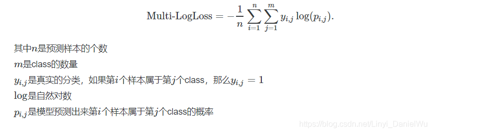
1.multi_logloss
def multiclass_logloss(actual, predicted, eps=1e-15):
    """Logarithmic Loss  Metric
    :param actual: 包含actual target classes的数组
    :param predicted: 分类预测结果矩阵, 每个类别都有一个概率
    """
    # Convert 'actual' to a binary array if it's not already:
    if len(actual.shape) == 1:
        actual2 = np.zeros((actual.shape[0], predicted.shape[1]))
        for i, val in enumerate(actual):
            actual2[i, val] = 1
        actual = actual2

    clip = np.clip(predicted, eps, 1 - eps)
    rows = actual.shape[0]
    vsota = np.sum(actual * np.log(clip))
    return -1.0 / rows * vsota
2.CountVectorizer()和TfidfVectorizer()计算方法介绍
https://blog.csdn.net/tang123246235/article/details/104528366
3.使用SVM,附著名的SVM 文章原理链接(花了一晚上还是没看懂数学部分)
不过这并不妨碍我开始用SVM:首先是对TF-IDF后的矩阵进行一个SVD降维操作:(找出对所有文本最重要的120个word)
然后对他进行归一化,之后进行SVM。
# Apply SVD, I chose 120 components. 120-200 components are good enough for SVM model.
svd = decomposition.TruncatedSVD(n_components=120)
svd.fit(xtrain_tfv)
xtrain_svd = svd.transform(xtrain_tfv)
xvalid_svd = svd.transform(xvalid_tfv)

# Scale the data obtained from SVD. Renaming variable to reuse without scaling.
scl = preprocessing.StandardScaler()
scl.fit(xtrain_svd)
xtrain_svd_scl = scl.transform(xtrain_svd)
xvalid_svd_scl = scl.transform(xvalid_svd)


clf = SVC(C=1.0, probability=True) # since we need probabilities
clf.fit(xtrain_svd_scl, ytrain)
predictions = clf.predict_proba(xvalid_svd_scl)

print ("logloss: %0.3f " % multiclass_logloss(yvalid, predictions))
但是最后效果不是特别好
4.遇事不绝,使用xgboost!!!
终于到了xgboost的环节,我知道自己再次看到这篇文章的时候对xgboost恐怕不会留下太深入的印象,下面是xgboost的对应文章:
入门加代码实现:
https://github.com/NLP-LOVE/ML-NLP/blob/master/Machine%20Learning/3.3%20XGBoost/3.3%20XGBoost.md
数学解析和详细解:
https://blog.csdn.net/v_JULY_v/article/details/81410574
这边同时还涉及到了稀疏函数的三种格式。 TfidfVectorizer()后的储存方式应该是csr矩阵,然后希望把他转换成csc进行运算
# Fitting a simple xgboost on tf-idf
clf = xgb.XGBClassifier(max_depth=7, n_estimators=200, colsample_bytree=0.8,
                        subsample=0.8, nthread=10, learning_rate=0.1)
clf.fit(xtrain_tfv.tocsc(), ytrain)
predictions = clf.predict_proba(xvalid_tfv.tocsc())

print ("logloss: %0.3f " % multiclass_logloss(yvalid, predictions))
5.网格搜索(Grid Search)
Its a technique for hyperparameter optimization. Not so effective but can give good results if you know the grid you want to use. I specify the parameters that should usually be used in this post: http://blog.kaggle.com/2016/07/21/approaching-almost-any-machine-learning-problem-abhishek-thakur/ Please keep in mind that these are the parameters I usually use. There are many other methods of hyperparameter optimization which may or may not be as effective.
In this section, I’ll talk about grid search using logistic regression.
Before starting with grid search we need to create a scoring function. This is accomplished using the make_scorer function of scikit-learn.
Grid Search:一种调参手段;穷举搜索:在所有候选的参数选择中,通过循环遍历,尝试每一种可能性,表现最好的参数就是最终的结果。其原理就像是在数组里找最大值。(为什么叫网格搜索?以有两个参数的模型为例,参数a有3种可能,参数b有4种可能,把所有可能性列出来,可以表示成一个3*4的表格,其中每个cell就是一个网格,循环过程就像是在每个网格里遍历、搜索,所以叫grid search)
https://www.cnblogs.com/wj-1314/p/10422159.html
基本技巧学习,本质就是穷举取最佳
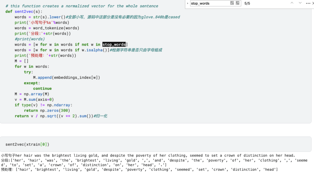
6.Word Vectors ,这里有两种方法,一种是 GloVe 一种是 word2vec,这里要复习一下词向量的定义
Tqdm 是一个快速,可扩展的Python进度条,可以在 Python 长循环中添加一个进度提示信息,用户只需要封装任意的迭代器
glove 可以直接用他的英文向量词库:glove.840B.300d.txt ,这个是840B tokens, 2.2M vocab, cased, 300d vectors
具体的NLP的内容之后我会再写个blog记录一下学习过程
word2vector 文章导航:
https://blog.csdn.net/kejizuiqianfang/article/details/99838249 这篇文章是word2vec的数学推导和对应多处理器的代码,讲的比较详细包含了具体的梯度更新方式强推!
这里附上数学推导的pdf版:
如果做中文的NLP还需要了解一下 jieba分词的package
这边是英文,直接调用 glove.840B.300d.txt
# load the GloVe vectors in a dictionary:

embeddings_index = {}
f = open('../input/glove840b300dtxt/glove.840B.300d.txt')
for line in tqdm(f):#tqdm是进度条模块
    values = line.split(" ")
    word = values[0]
    coefs = np.asarray(values[1:], dtype='float32')
    embeddings_index[word] = coefs
f.close()
#embedding 对每个word vector 加载对应的三百维 的变量
print('Found %s word vectors.' % len(embeddings_index))
然后对每个句子产生归一化的300维的句向量
到这里为止,传统机器学习部分就结束了,然后是神经网络部分的内容:
首先是LSTM处理,LSTM是老朋友了,可以算得是RNN里面的万金油了,这里是用keras来实现的,关于LSTM,主要相对于RNN提升了两个方面的表现,一个是NLP中的 long dependency, 另一个是他的cell state在继承之前的状态时使用了更多的加法减少了梯度衰退的速度。我不认为你下次碰到这篇文章时会连lstm都记不清了,但以防万一,这里附上经典原理实现版的jupyter notebook.由于安全性的原因不能上传ipynb,记得改后缀。
这部分主要着眼于数据的处理,非常有意思。
首先是最简单的神经网络,对输入量进行处理:多分类任务首先要把label 变为一维向量:to_categorical,对输入X正态化
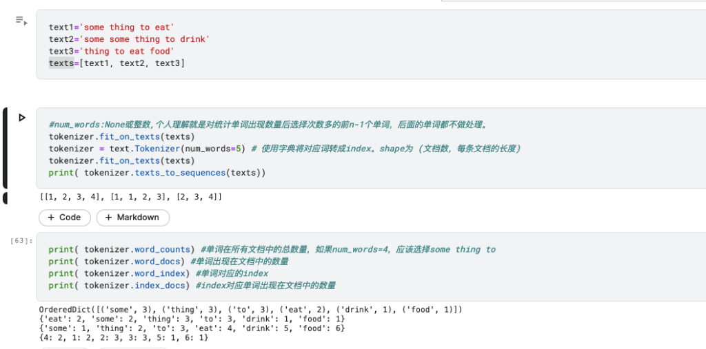
对lstm输入文本首先要进行文本序列化:一个简单的例子
https://blog.csdn.net/qq_16234613/article/details/79436941
另一个有趣的技巧是early stopping.在call back的时候,如果达到了最佳状态,就停止:
# A simple LSTM with glove embeddings and two dense layers
model = Sequential()
model.add(Embedding(len(word_index) + 1,
                     300,
                     weights=[embedding_matrix],
                     input_length=max_len,
                     trainable=False))
model.add(SpatialDropout1D(0.3))
model.add(LSTM(300, dropout=0.3, recurrent_dropout=0.3))

model.add(Dense(1024, activation='relu'))
model.add(Dropout(0.8))

model.add(Dense(1024, activation='relu'))
model.add(Dropout(0.8))

model.add(Dense(3))
model.add(Activation('softmax'))
model.compile(loss='categorical_crossentropy', optimizer='adam')

# Fit the model with early stopping callback
earlystop = EarlyStopping(monitor='val_loss', min_delta=0, patience=3, verbose=0, mode='auto')
model.fit(xtrain_pad, y=ytrain_enc, batch_size=512, epochs=100,
          verbose=1, validation_data=(xvalid_pad, yvalid_enc), callbacks=[earlystop])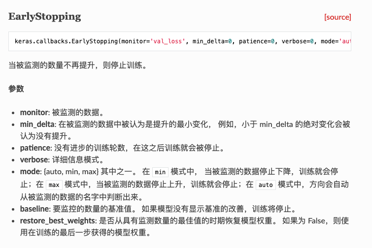
值得注意的是,这里有一个可以优化的地方,就是不要用原文中的Embedding层训练词向量矩阵,最好用已经预训练过的结果,具体可以参考
https://github.com/MoyanZitto/keras-cn/blob/master/docs/legacy/blog/word_embedding.md
GRU类似与之类似,kaggle上的这个code最有意思的地方是他简洁注释清晰的模型集成(Model Ensembling)代码。之后我自己照着写一遍,记录一下感受,现在懒得写了,毕设的ppt还没动😢。
开始复现了一遍,本质上是一个非常简单的双层stacking 模型。
# specify the data to be used for every level of ensembling:
train_data_dict = {0: [xtrain_tfv, xtrain_ctv, xtrain_tfv,xtrain_ctv, xtrain_glove], 1: []}
test_data_dict = {0: [xvalid_tfv, xvalid_ctv, xvalid_tfv,xtrain_ctv, xvalid_glove], 1: []}

model_dict = {0: [LogisticRegression(), LogisticRegression(), MultinomialNB(alpha=0.1),MultinomialNB(),xgb.XGBClassifier(silent=True, n_estimators=120, max_depth=7)],

              1: [LogisticRegression()]}

ens = Ensembler(model_dict=model_dict, num_folds=3, task_type='classification',
                optimize=multiclass_logloss, lower_is_better=True, save_path='')

ens.fit(train_data_dict, ytrain, lentrain=xtrain_ctv.shape[0])
preds = ens.predict(test_data_dict, lentest=xvalid_ctv.shape[0])
具体实现是第一层输入用交叉验证训练多个模型将交叉验证的结果保存为下一层的xtrain, 然后见
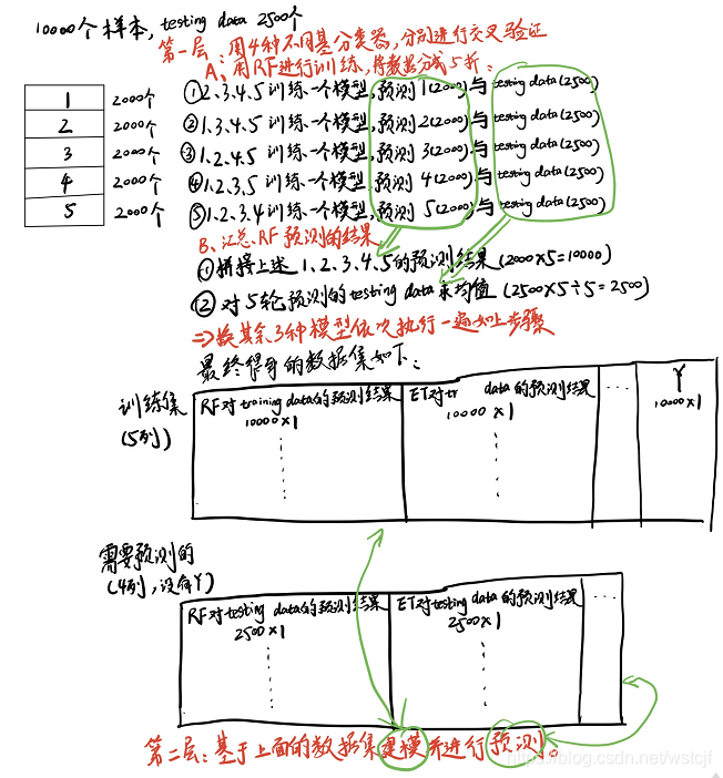
值得注意的是,原文中于stacking方法有一小点不同,原文中不是五轮test取平均,而是直接用fit整个traindata然后得到的predict的test_prob做下一层的testdata,但是fit和predict更容易分离。
本文只是简单的就Kaggle上面的那篇文章梳理了上面提到过的知识点,而那篇文章由于当时的时代局限性还有相当多的方法没有涉及。最起码在机器学习方面没有涉及到LDA等主题模型,各种花式的HMM,RNN方面没有涉及各类变种LSTM,( BiLSTM, Hierarchical LSTM)还有各种各样的优化技巧,没有涉及到神经网络中的CNN,attention,强化学习。除了word embeding 外其他可行的文本特征预处理(BERT, ELMO,GPT),多线程方面的加速技巧,甚至于一些奇淫巧技(用GAN做文本增强 等)都还没有涉及到。如果未来的我如果以后吃这碗饭(大概率不会)可以接着找资料记录一下学习过程。就这样,留个档。


 489
489


 被折叠的 条评论
为什么被折叠?
被折叠的 条评论
为什么被折叠?
 到【灌水乐园】发言


