线性逻辑回归logistic regression

逻辑回归

1. 垃圾邮件分类
2. 测试肿瘤是良性还是恶性
3. 预测某人的信用是否良好

Sigmoid/Logistic Function
θ和x是矩阵类型的，θ是参数矩阵，x是数据矩阵

g(x)的取值范围是0—1，就可以分为两类，大于0.5为1类，小于0.5为另一类。

决策边界

中间这条线是值为零的等高线。

画一个圆，半径为1，这就是一个决策边界。

很复杂的决策边界。

逻辑回归的代价函数：
h(X)是样本值，y是标签值。
就是0，1两类代价函数的不同表达。

分段函数合并在一个表达式之中：
要对θ进行求导：

求导过程：

逻辑回归一般来说是做二分类的问题的。

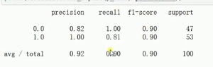
正确率、召回率，F1指标

举个例子：

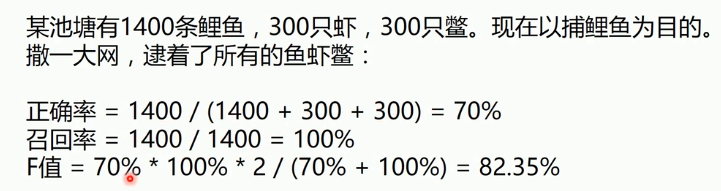
F1指标的真正的公式：

梯度下降法的逻辑回归

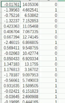
数据：

import matplotlib.pyplot as plt
import numpy as np
from sklearn.metrics import classification_report
from sklearn import preprocessing
#数据是否需要标准化
scale=False

#载入数据
data = np.genfromtxt("LR-testSet.csv",delimiter=',')
x_data = data[:,:-1]
y_data = data[:,-1]

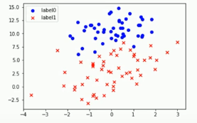
def plot():
    x0=[]
    x1=[]
    y0=[]
    y1=[]
    #切分不同类别的数据,一行一行的判别
    for i in range(len(x_data)):
        if y_data[i]==0:
            x0.append(x_data[i,0])
            y0.append(x_data[i,1])
        else:
            x1.append(x_data[i, 0])
            y1.append(x_data[i, 1])

    #画图（散点图）
    scatter0 = plt.scatter(x0,y0,c='b',marker='o')#实心圆点
    scatter1 = plt.scatter(x1, y1, c='r', marker='x')#画叉点
    #画图例（上方说明）
    plt.legend(handles=[scatter0,scatter1],labels=['label0','label1'],loc='best')

plot()#绘制二维图像
plt.show()#打印出来

#数据处理，添加偏置值
x_data = data[:,:-1]
y_data = data[:,-1,np.newaxis]

print(np.mat(x_data).shape)#(100,2)
print(np.mat(y_data).shape)#(100,1)
#给样本添加偏置值
X_data = np.concatenate((np.ones(100,1),x_data),axis=1)
print(X_data.shape)#(100,3)

def sigmoid(x) :
    return 1.0/(1+np.exp(-x))

#ws权值矩阵θ，按位相乘
def cost(xMat,yMat,ws):
    left = np.multiply(yMat,np.log(sigmoid(xMat*ws)))
    right = np.multiply(1-yMat,np.log(1-sigmoid(xMat*ws)))
    return np.sum(left+right)/-(len(xMat))

def gradAscent(xArr,yArr):
    #是否要做数据标准化
    if scale == True:
        xArr = preprocessing.scale(xArr)
    xMat = np.mat(xArr)
    yMat = np.mat(yArr)

    lr=0.001
    epochs = 10000
    costList=[]
    #计算数据行列数
    #把矩阵行列值得到，行代表数据个数，列代表权值个数
    m,n = np.shape(xMat)#值为100和3
    #初始化权值
    ws = np.mat(np.ones((n,1)))

    #在迭代过程中ws是在改变着的
    for i in range(epochs+1):
        #xMat和weights矩阵相乘
        h=sigmoid(xMat*ws)
        #计算误差，代价函数，得到三行一列的矩阵
        ws_grad = xMat.T*(h-yMat)/m
        ws = ws-lr*ws_grad
        #每迭代50次保存一下cost值
        if i % 50 == 0:
            costList.append(cost(xMat,yMat,ws))
    return ws,costList
#训练模型，得到权值和cost的变化
ws,costList = gradAscent(X_data,y_data)
print(ws)

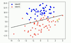
#决策边界 w[0]+w[1]x1+w[2]x2
if scale == False :
    plot()
    x_test = [[-4],[3]]
    y_test = (-ws[0]-x_test*ws[1])/ws[2]
    plt.plot(x_test,y_test,'k')
    plt.show()
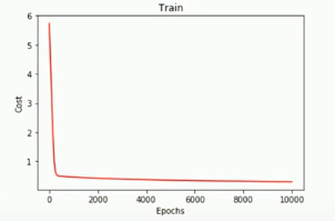
#画图loss值的变化
x = np.linspace(0,10000,201)
plt.plot(x,costList,c='r')
plt.title('Train')
plt.xlabel('Epochs')
plt.ylabel('Cost')
plt.show()

#预测
def predict(x_data,ws):
    if scale == True:
        x_data = preprocessing.scale(x_data)
        xMat = np.mat(x_data)
        ws = np.mat(ws)
        return [1 if x>=0.5 else 0 for x in sigmoid(xMat*ws)]
predictions = predict(X_data,ws)
predict(classification_report(y_data,predictions))

打印出的ws的值

分界线：

loss值的变化：记录了201次

准确率、召回率

如果数据标准化设置为true的画，loss值变化会缓慢，得到的cost值比较高一点。

调用sklean的逻辑回归完成程序

import matplotlib.pyplot as plt
import numpy as np
from sklearn.metrics import classification_report
from sklearn import preprocessing
from sklearn import linear_model
#数据是否需要标准化
scale=False

#载入数据
data = np.genfromtxt("LR-testSet.csv",delimiter=',')
x_data = data[:,:-1]
y_data = data[:,-1]

def plot():
    x0=[]
    x1=[]
    y0=[]
    y1=[]
    #切分不同类别的数据,一行一行的判别
    for i in range(len(x_data)):
        if y_data[i]==0:
            x0.append(x_data[i,0])
            y0.append(x_data[i,1])
        else:
            x1.append(x_data[i, 0])
            y1.append(x_data[i, 1])

    #画图（散点图）
    scatter0 = plt.scatter(x0,y0,c='b',marker='o')#实心圆点
    scatter1 = plt.scatter(x1, y1, c='r', marker='x')#画叉点
    #画图例（上方说明）
    plt.legend(handles=[scatter0,scatter1],labels=['label0','label1'],loc='best')

plot()#绘制二维图像
plt.show()#打印出来

logistic = linear_model.LogisticRegression()
logistic.fit(x_data,y_data)
#决策边界 w[0]+w[1]x1+w[2]x2
if scale == False :
    plot()
    x_test = np.array([[-4],[3]])
    #intercept偏置  coef是权值，模型参数，二维的，两个特征值，所以是两个参数
    y_test = (-logistic.intercept_-x_test*logistic.coef_[0][0])/logistic.coef_[0][1]
    plt.plot(x_test,y_test,'k')
    plt.show()

predictions = logistic.predict(x_data)
print(classification_report(y_data,predictions))