


目录
谱聚类
谱聚类的特点
• 1.对数据的结构没有假设(适应性广)
• 2 经过特殊的构图处理后计算很快
• 3.不会像kmeans一样将一些离散的小簇聚在一起
•
1.对于不同的构图方式比较敏感
•
2.对于超参数设置比较敏
谱聚类整体思路

构图
•
根据训练集,计算相似度矩阵
• 根据相似度矩阵采用某种构图方法计算w权重矩阵
• 根据w权重矩阵计算D矩阵和拉普拉斯矩阵
相似度矩阵
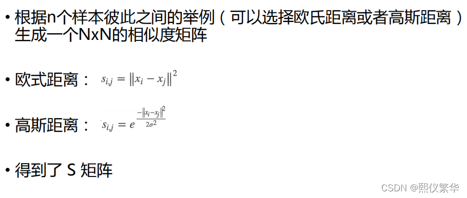
根据构图方式计算W矩阵

1

2

3

计算D矩阵和拉普拉斯矩阵

切图

切图目的

Ratia Cut

分图方法

谱聚类探索
# !/usr/bin/python
# -*- coding:utf-8 -*-

import numpy as np
import matplotlib.pyplot as plt
import matplotlib.colors
from sklearn.cluster import spectral_clustering
from sklearn.metrics import euclidean_distances


def expand(a, b):
    d = (b - a) * 0.1
    return a-d, b+d


if __name__ == "__main__":
    matplotlib.rcParams['font.sans-serif'] = [u'SimHei']
    matplotlib.rcParams['axes.unicode_minus'] = False

    t = np.arange(0, 2*np.pi, 0.1)
    data1 = np.vstack((np.cos(t), np.sin(t))).T
    data2 = np.vstack((2*np.cos(t), 2*np.sin(t))).T
    data3 = np.vstack((3*np.cos(t), 3*np.sin(t))).T
    data = np.vstack((data1, data2, data3))

    n_clusters = 3
    m = euclidean_distances(data, squared=True)
    sigma = np.median(m)

    plt.figure(figsize=(12, 8), facecolor='w')
    plt.suptitle(u'谱聚类', fontsize=20)
    clrs = plt.cm.Spectral(np.linspace(0, 0.8, n_clusters))
    for i, s in enumerate(np.logspace(-2, 0, 6)):
        print(s)
        af = np.exp(-m ** 2 / (s ** 2)) + 1e-6
        y_hat = spectral_clustering(af, n_clusters=n_clusters, assign_labels='kmeans', random_state=1)
        plt.subplot(2, 3, i+1)
        for k, clr in enumerate(clrs):
            cur = (y_hat == k)
            plt.scatter(data[cur, 0], data[cur, 1], s=40, c=clr, edgecolors='k')
        x1_min, x2_min = np.min(data, axis=0)
        x1_max, x2_max = np.max(data, axis=0)
        x1_min, x1_max = expand(x1_min, x1_max)
        x2_min, x2_max = expand(x2_min, x2_max)
        plt.xlim((x1_min, x1_max))
        plt.ylim((x2_min, x2_max))
        plt.grid(True)
        plt.title(u'sigma = %.2f' % s, fontsize=16)
    plt.tight_layout()
    plt.subplots_adjust(top=0.9)
    plt.show()

聚类跟图片数据探索:
# !/usr/bin/python
# -*- coding: utf-8 -*-

from PIL import Image
import numpy as np
from sklearn.cluster import KMeans
import matplotlib
import matplotlib.pyplot as plt
from mpl_toolkits.mplot3d import Axes3D


def restore_image(cb, cluster, shape):
    row, col, dummy = shape
    image = np.empty((row, col, 3))
    index = 0
    for r in range(row):
        for c in range(col):
            image[r, c] = cb[cluster[index]]
            index += 1
    return image


def show_scatter(a):
    N = 10
    print('原始数据:\n', a)
    density, edges = np.histogramdd(a, bins=[N,N,N], range=[(0,1), (0,1), (0,1)])
    density /= density.max()
    x = y = z = np.arange(N)
    d = np.meshgrid(x, y, z)

    fig = plt.figure(1, facecolor='w')
    ax = fig.add_subplot(111, projection='3d')
    ax.scatter(d[1], d[0], d[2], c='r', s=100*density, marker='o', depthshade=True)
    ax.set_xlabel(u'红色分量')
    ax.set_ylabel(u'绿色分量')
    ax.set_zlabel(u'蓝色分量')
    plt.title(u'图像颜色三维频数分布', fontsize=20)

    plt.figure(2, facecolor='w')
    den = density[density > 0]
    den = np.sort(den)[::-1]
    t = np.arange(len(den))
    plt.plot(t, den, 'r-', t, den, 'go', lw=2)
    plt.title(u'图像颜色频数分布', fontsize=18)
    plt.grid(True)

    plt.show()


if __name__ == '__main__':
    matplotlib.rcParams['font.sans-serif'] = [u'SimHei']
    matplotlib.rcParams['axes.unicode_minus'] = False

    num_vq = 20
    im = Image.open('../data/Lena.png')     # flower2.png(200)/lena.png(50)
    image = np.array(im).astype(np.float) / 255
    image_v = image.reshape((-1, 3))
    model = KMeans(num_vq)
    show_scatter(image_v)

    N = image_v.shape[0]    # 图像像素总数
    # 选择足够多的样本(如1000个),计算聚类中心
    idx = np.random.randint(0, N, size=1000)
    image_sample = image_v[idx]
    model.fit(image_sample)
    c = model.predict(image_v)  # 聚类结果
    print('聚类结果:\n', c)
    print('聚类中心:\n', model.cluster_centers_)

    plt.figure(figsize=(15, 8), facecolor='w')
    plt.subplot(121)
    plt.axis('off')
    plt.title(u'原始图片', fontsize=18)
    plt.imshow(image)
    # plt.savefig('1.png')

    plt.subplot(122)
    vq_image = restore_image(model.cluster_centers_, c, image.shape)
    plt.axis('off')
    plt.title(u'矢量量化后图片:%d色' % num_vq, fontsize=20)
    plt.imshow(vq_image)
    # plt.savefig('2.png')

    plt.tight_layout(1.2)
    plt.show()
D:\ProgramData\Anaconda3\envs\data_analys\python.exe D:/worke/pycode/PCA/20190713/cluster_images.py
原始数据:
 [[0.87058824 0.53333333 0.48235294]
 [0.87843137 0.54117647 0.49019608]
 [0.89019608 0.54509804 0.49803922]
 ...
 [0.68235294 0.26666667 0.31372549]
 [0.70588235 0.2745098  0.31764706]
 [0.74117647 0.30588235 0.34117647]]
聚类结果:
 [17 11 11 ... 10 10  3]
聚类中心:
 [[0.8212766  0.57613684 0.5612015 ]
 [0.56655568 0.20207177 0.28642249]
 [0.37235927 0.10664137 0.2771031 ]
 [0.74977557 0.3265769  0.3448618 ]
 [0.94977376 0.80708899 0.62518854]
 [0.7872549  0.50157952 0.48022876]
 [0.48413547 0.27789661 0.47771836]
 [0.60371517 0.39153767 0.57254902]
 [0.43719165 0.19253637 0.36824794]
 [0.90933707 0.78347339 0.72679739]
 [0.67575953 0.25770308 0.30644258]
 [0.91372549 0.59200603 0.47903469]
 [0.82413273 0.39495798 0.38866624]
 [0.93246187 0.72701525 0.5204793 ]
 [0.86887255 0.68611111 0.64133987]
 [0.4504902  0.13145425 0.26062092]
 [0.70916799 0.40370959 0.44705882]
 [0.87671569 0.49129902 0.43498775]
 [0.33754325 0.06482122 0.22537486]
 [0.60090498 0.29864253 0.36983409]]
D:/worke/pycode/PCA/20190713/cluster_images.py:84: MatplotlibDeprecationWarning: Passing the pad parameter of tight_layout() positionally is deprecated since Matplotlib 3.3; the parameter will become keyword-only two minor releases later.
  plt.tight_layout(1.2)

Process finished with exit code 0


 3万+
3万+


 被折叠的 条评论
为什么被折叠?
被折叠的 条评论
为什么被折叠?
 到【灌水乐园】发言


