【基础内容：卷积神经+plt.subplots子图功能+数组的双循环遍历】卷积核的python程序设计生成代码段

理解从卷积核数组中提取及进行求和后的新数组生成过程。

1. 知识框架—定义数组
2. 知识框架–数组取数
3. 知识框架—数组写入plt画布
4. 知识框架—卷积结果的维度表示: 原数组长度 - 卷积数组长度-1
   5. 知识难点—理解如何利用i,j从filter数组中提取每1位置的数字
   6.知识难点—image[i:i+filter.shape[0],j:j+filter.shape[1]] * filter，代码的含义理解

难点解析

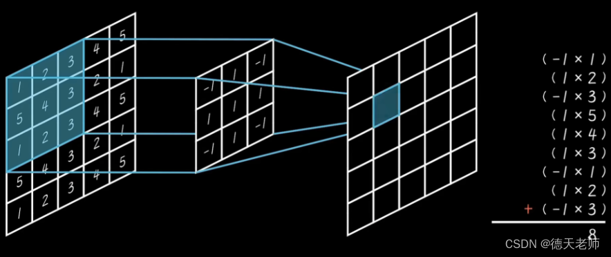
np.sum(image[i:i+filter.shape[0],j:j+filter.shape[1]] * filter)理解此处代码(图中数据与示例不符，但原理相同)，请参考下图：
第1个图：featuremap
第2个图：filter

import numpy as np
ori_Num = np.array([[1,3,4,0,1],
         [6,6,0,1,2],
         [1,2,4,2,0],
         [3,4,3,0,1],
         [2,0,1,5,2]])

#卷积核提取
filter = np.array([[2,5,0],
                 [0,1,3],
                 [1,0,2]])
for i in range(filter.shape[0]):
    for j in range(filter.shape[0]):

        if i == 0 and j == 0:
            print('-'*10)
        elif i == 1 and j == 0:
            print('-'*10)

        elif i == 2 and j == 0:
            print('-'*10)
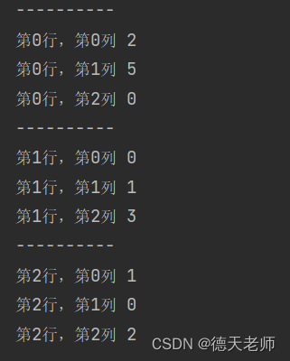
        print(f'第{i}行，第{j}列', filter[i, j])

输出效果图：

通过卷积核的卷积运行得到新的结论数组

1. 上段代码中，能够帮助大家更好的理解def conv(image,filter)中对于源数组的求和运算featuremap
2. 在函数conv中featuremap—image,是同一组数据。

"""本示例结合卷积神经网络的卷积核生成以图形化的方式展示如何确定卷积核"""
import numpy as np
import matplotlib.pyplot as plt
plt.rcParams['font.sans-serif']=['SimHei'] # 用来正常显示中文标签
plt.rcParams['axes.unicode_minus']=False # 用来正常显示负号


def conv(image,filter):
    '''       i=0时image取数数组：
           ----i范围：0~3   j范围：0~3，
               *i取0时：
                   ：j取0:0+3
                   ：image[0:3,0:3]

                   ：j取1时，
                    image[0:3,1:4]

                   j取2时，：
                   image[0:3,2:5]
            *i取1时：
                   ：j取0:
                   ：image[1:4,0:3]

                   ：j取1时，
                    image[1:4,1:4]

                   j取2时，：
                   image[1:4,2:5]

            *i取2时：
                   ：j取0:
                   ：image[2:5,0:3]

                   ：j取1时，
                    image[2:5,1:4]

                   j取2时，：
                   image[2:5,2:5]


              np.sum()对数组的多行，多列求和法。

               '''
    #print('shape[0]',image.shape[1])
    print(image.shape[0]-(filter.shape[0]-1))

    result = []
    #取到image行列数为5,同时取filter行数3两者差为2
    for i in range(image.shape[0]-(filter.shape[0]-1)): #取原数组和卷积核的行-1的差，i=5-2=3[0,1,2]
        for j in range(image.shape[1]-(filter.shape[1]-1)): #取原数组和卷积核的列-1差,j=5-2=3[0,1,2]

            value = np.sum(image[i:i+filter.shape[0],j:j+filter.shape[1]] * filter)
            result.append(value)
    result = np.array(result)
    res = result.reshape(image.shape[0]-filter.shape[0]+1,image.shape[1]-filter.shape[1]+1)
    return res


#卷积前数组 featuremap.shap[0],行长度值=5
featuremap = np.array([[1,3,4,0,1],
         [6,6,0,1,2],
         [1,2,4,2,0],
         [3,4,3,0,1],
         [2,0,1,5,2]])
#卷积核 filter.shape[0],行长度值=3
filter = np.array([[2,5,0],
                 [0,1,3],
                 [1,3,2]])
#运行卷积后求和的新数组result = [3，3] 3行，3列
result = conv(featuremap,filter)
#print(result[0,0]) #result是一个3行，3列的二维数组，所以可以通过result[0,0]的方式，for循环中依次取出

#把卷积后的结果数组，通过plt画布写出来
fig, axes = plt.subplots(3, 3)
fig.subplots_adjust(wspace=0,hspace=0)#0.01~0.09之间比较合适
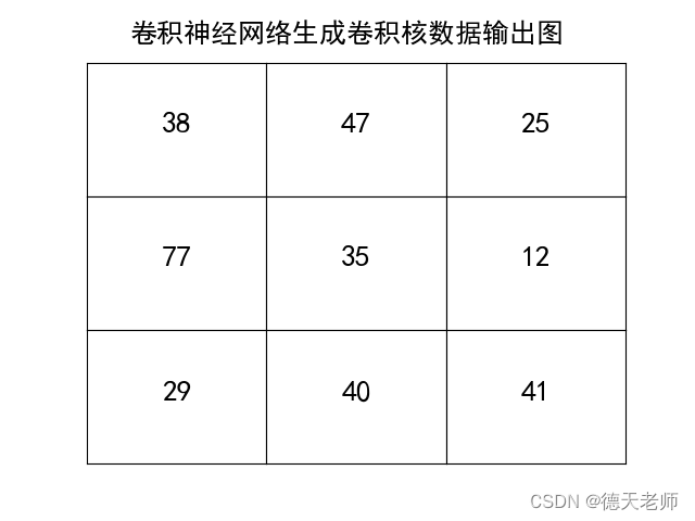
fig.suptitle('卷积神经网络生成卷积核数据输出图',y=0.96,fontsize=18)#y值取0.01~0.99之间过大超界

for i in range(0,3):
    for j in range(0,3):
        #通过设置子图的主题，把生成的二维数组依次取出写到子图内部。
        axes[i][j].set_title(f'{result[i][j]}',x=0.5,y=0.4,fontsize=20)#位置调节，数据向上y值变大，数据向右x变大，数据范围0~0.9合适
        axes[i,j].axes.yaxis.set_visible(False)

        axes[i,j].xaxis.set_visible(False)


plt.show()