ACSE8 L1

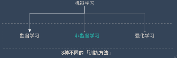
Machine learning

definition

A computer program is said to learn from experience E with respect to some task T and some performance measure P if its performance on T, as measured by P, improves with experience E.

2. 例子
   基于一个包含60,000个带标签的数字图像的训练集（体验E），学习一种算法，该算法在给定新的像素化输入图像后，会自动识别出它代表的数字（任务T）。 性能P量化了10,000张图像测试集上算法的准确性
   
3. Supervised vs Unsupervised Learning
   

Supervised Learning

1. 定义

task T is clearly defined because the data are labeled and the computer has to predict the labels of new data. Performance P is quantified by the mismatch between predicted and actual labels of new data

2. 流程

监督学习需要有明确的目标，很清楚自己想要什么结果。比如：按照“既定规则”来分类、预测某个具体的值…
（1）选择一个适合目标任务的数学模型
（2） 先把一部分已知的“问题和答案”（训练集）给机器去学习
（3） 机器总结出了自己的“方法论”
（4）人类把”新的问题”（测试集）给机器，让他去解答

下面这个例子更方便理解
假如我们想要完成文章分类的任务，则是下面的方式：
（1） 选择一个合适的数学模型
（2） 把一堆已经分好类的文章和他们的分类给机器
（3）机器学会了分类的“方法论”
（4） 机器学会后，再丢给他一些新的文章（不带分类），让机器预测这些文章的分类

3. Regression

1. 回归：预测连续的、具体的数值。比如：支付宝里的芝麻信用分数
2. 例子：卖酸奶
   
   Task T: from the Training Set of pairs (Temperature, Yoghurt Sold) (the Experience)建立一个公式，用于仅在知道Temperature的情况下预测 Yoghurt Sold (the Task) 以使averaged squared error最小(the Performance))

Linear Regression

定义

回归是通过历史数据，摸透了“套路”，然后通过这个套路来预测未来的结果。
线性关系不仅仅只能存在 2 个变量（二维平面）。3 个变量时（三维空间），线性关系就是一个平面，4 个变量时（四维空间），线性关系就是一个体。以此类推…

（2） Standard ML Terminology & Notations

m = number of training examples (here we have m = 50 pairs of data)
x’s = input variables/features (here x is just depth)
y’s = output variables/target variables (here y is porosity)
$(x^{(i)},y^{(i)})$ is the $i^{th}$ training example

What does Linear Regression do?

1. Fit a linear function to the data. In Machine Learning terminology, this function is called the « Hypothesis »$h_{\theta }(x)$
   $$h_{\theta }(x)={\theta }_0+{\theta }_{1}x$$
   ${\theta }_0$ and ${\theta }_1$ are called the parameters (or the weights) of the model.
2. For each value of the feature $x^i$ in the Training Set , we want $h_{\theta }(x^i)$ to be close to the target $y^i$ . In other words, we wish to minimize the Loss Function $J({\theta }_0,{\theta }_1)$ (also called Cost Function).
   
3. 当 « Bias » term ${\theta }_0$ 为0时
   $$h_{\theta }(x)={\theta }_{1}x$$
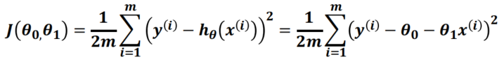
   The loss function $J({\theta }_0,{\theta }_1)$ becomes
   
   The loss function is simply a second degree polynomial in ${\theta }_1$, minimum for
   
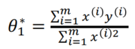
   This is called normal equation
   (2) Loss Function is Convex for Regression
   
   (3) Gradient Descent on a Convex Function
   

• $\alpha$ is the learning rate, fixed by the user.
• If $\alpha$ is too small , convergence can be too slow, if $\alpha$ is too large it may miss the minimum.

4. 当有Bias Term时, linear regression 的cost function是
   The cost function $J({\theta }_0,{\theta }_1)$ can be easily developed
   
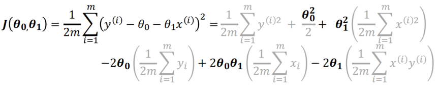
   The cost function is simply a second degree polynomial in ${\theta }_0$ and ${\theta }_1$. It reaches its minimum for the values of ${\theta }_0$and ${\theta }_1$ given by the normal equations
   
   (2) Cost Function for ${\theta }_0$ and ${\theta }_1$

A nice property of a convex cost function 是它没有局部最小值。 如果您无法再减小损失函数，则表明您已达到全局最小值。但是, many cost functions in non-linear problems are non-convex

优缺点

1. 优点
   (1) 建模速度快，不需要很复杂的计算，在数据量大的情况下依然运行速度很快。
   (2) 可以根据系数给出每个变量的理解和解释
2. 缺点
   不能很好地拟合非线性数据。所以需要先判断变量之间是否是线性关系。

Multiple Linear Regression

定义

$$h_{\theta }(x_1,x_{2,}.....x_n)={\theta }_0+{\theta }_1{x}_1+{\theta }_2{x}_2....+{\theta }_n{x}_n$$

$y^{(i)}$is the value of the target in the example i of the training set
$x_j^{(i)}$ is the value of the feature j in the example i of the training set
$m$ is the number of examples in the training set
$n$ is the number of features in each example of the training set

例子

根据平方尺，卧室数量，浴室数量，…来预测房价
根据父母双方的大小，营养，环境因素……预测孩子的身高

Vector Notation for Multiple Linear Regression

The hypothesis function is, if we have $n$ input features $x_i$:
$$y=h_{\theta }(x_1,x_{2,}.....x_n)={\theta }_0+{\theta }_1{x}_1+{\theta }_2{x}_2....+{\theta }_n{x}_n$$
With the vector notation $x=\left(\begin{array}{c}\begin{array}{c}1\\ x_1\\ ...\end{array}\\ x_n\end{array}\right)$, $\theta =\left(\begin{array}{c}\begin{array}{c}1\\ {\theta }_1\\ ...\end{array}\\ {\theta }_n\end{array}\right)$, We have $h_{\theta }(x)={\theta }^{T}x$.
We write the $m$ data vectors as: $(x^{(i)},y^{(i)})$, $x^{(i)}=\left(\begin{array}{c}\begin{array}{c}{x}_1^{(i)}\\ x_2^{(i)}\\ \dots \end{array}\\ x_n^{(i)}\end{array}\right)$ and $y^{(i)}$ real for i = 1,…m

Logistic Regression

定义

这个算法是分类算法, 我们希望想出一个满足某个性质的假设函数，这个性质是它的预测值要在0和1之间。
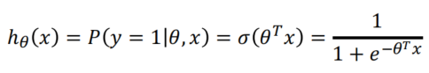
我们引入一个新的模型，逻辑回归，该模型的输出变量范围始终在0和1之间。 逻辑回归模型的假设是： $h_{\theta }(x)=\sigma ({\theta }^{T}X)$
其中： X 代表特征向量, $\sigma$ 代表逻辑函数（logistic function)是一个常用的逻辑函数为S形函数（Sigmoid function），公式为：$\sigma (z)=\frac{1}{1+e^{-z}}$
$h_{\theta }(x)$的作用是，对于给定的输入变量，根据选择的参数计算输出变量=1的可能性（estimated probablity）即$h_{\theta }(x)=P(y=1|\theta ,x)$
（2） Sigmoid Function for transformation to [0,1] domain
The Sigmoid function $\sigma (z)$ is also called the Logistic Function. It transforms a real value $z$ into a value between 0 and 1

$$\sigma (z)=\frac{1}{1+e^{-z}}$$
A useful equation is: ${\sigma }^{{}^{\prime }}(z)=(1-\sigma (z))\sigma (z)$

Interpreting the output of the Logistic function

Say that $y$ is the outcome of a regression equation for an input $x$
$$y={\theta }_0+{\theta }_1{x}_1+{\theta }_2{x}_2+.....+{\theta }_n{x}_n$$
In vector form
$$y={\theta }^{T}x$$
$y$ is a real number which can take any positive or negative value
If we apply the sigmoid (or logistic) function $\sigma (y)$ we obtain a value between 0 and 1, which we interpret as the probability for the class to be 1

$h_{\theta }(x)$ is interpreted as a probability between 0 and 1. Hence the predicted class for a new feature vector $x$ will be:

Decision Boundary

1. 这个概念能更好地帮助我们理解逻辑回归的假设函数在计算什么
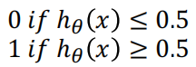
   在逻辑回归中, 我们预测
   当$h_{\theta }(x)>=0.5$时, 预测 y=1
   当$h_{\theta }(x)<0.5$ 时, 预测 y=0
   根据上面绘制出的 S 形函数图像，我们知道当
   z = 0 时, $\sigma (z)=0.5$
   z > 0 时, $\sigma (z)>0.5$
   z < 0 时, $\sigma (z)<0.5$
   又因为 $z={\theta }^{T}x$, 即
   ${\theta }^{T}x>=0$时, 预测 y=1
   ${\theta }^{T}x<0$时, 预测 y=0
2. 现在假设我们有一个模型：
   
   $$h_{\theta }(x)=\sigma ({\theta }_0+{\theta }_1{x}_1+{\theta }_2{x}_2)$$
   并且参数θ 是向量[-3 1 1]。 则当$-3+x_1+x_2\ge 0$，即$x_1+x_2\ge 3$时，模型将预测 y=1。 我们可以绘制直线$x_1+x_2=3$，这条线便是我们模型的分界线，将预测为1的区域和预测为 0的区域分隔开。Hence the Decision Boundary in 2D is the line of equation ${\theta }^{T}x=0$
   
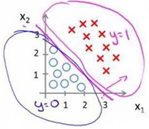
   决策边界是假设函数的一个属性, 它包括${\theta }_0,{\theta }_1,{\theta }_2$. 在上张图中,我画了一个训练集和一组数据使其可视化, 但是即使我们去掉数据集. 这条决策边界以及我们预测y = 0和y=1的区域, 之后我们采用数据训练集得到参数θ。 一旦我们确定参数θ, 我们将完全确定决策边界，这时我们不需要通过绘制训练集来确定决策边界

Cost Function for Logistic Regression

1. One data point
   For one data point , how to measure the
   discrepancy(差异) between the actual data value y (equal to 0 or 1) and the estimated probability $h_{\theta }(x)$ ?
   
   
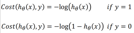
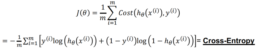
   Combining the two possibilities above into one single equation:
   $$Cost(h_{\theta }(x),y)=-y\log ((h_{\theta }(x))-(1-y)\log (1-(h_{\theta }(x))$$

2. whole Set $((x^{(i)}),(y^{(i)}))$ i=1,…m
   
   To minimize, just calculate the derivatives $\frac{\partial J(\theta )}{\partial {\theta }_j}$ for j = 1,…n and apply Gradient Descent
   $$\frac{\partial J(\theta )}{\partial {\theta }_j}=\frac{1}{m}\sum _{i=1}^m[h_{\theta }(x^{(i)})-y^{(i)}]x_j^{(i)}$$
   证明过程网址: https://math.stackexchange.com/questions/477207/derivative-of-cost-function-for-logistic-regression
   Logistic Regression 用于分类而不是回归

Simple Example of Non-Linear Logistic Regression

The m= 1000 data points $(x_1^i,x_2^i{)}_{i=1000}$ are in the plane. A group of data are one color, the other group another color.
Question: predict the color at each location of the plane.

Model used for Logistic Regression:

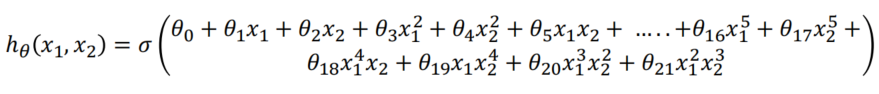
Decision Boundary will be a polynomial of degree 5.

2. Configurations for Non-Linear Logistic Regression

Will have to decide which polynomial degree is statistically reasonable and which one is too high and causes “overfitting”
将必须决定哪个多项式在统计上是合理的，哪个多项式太高而导致“过度拟合”（如第三个示例所示）

4.Classification

1. 分类：对各种事物分门别类，用于离散型预测

5. 主流的监督学习算法

算法	类型	简介
朴素贝叶斯	分裂	贝叶斯分类法是基于贝叶斯定定理的统计学分类方法。它通过预测一个给定的元组属于一个特定类的概率，来进行分类。朴素贝叶斯分类法假定一个属性值在给定类的影响独立于其他属性的 —— 类条件独立性。
决策树	分类	决策树是一种简单但广泛使用的分类器，它通过训练数据构建决策树，对未知的数据进行分类。
SVM	分类	支持向量机把分类问题转化为寻找分类平面的问题，并通过最大化分类边界点距离分类平面的距离来实现分类。
逻辑回归	分类	逻辑回归是用于处理因变量为分类变量的回归问题，常见的是二分类或二项分布问题，也可以处理多分类问题，它实际上是属于一种分类方法
线性回归	回归	线性回归是处理回归任务最常用的算法之一。该算法的形式十分简单，它期望使用一个超平面拟合数据集（只有两个变量的时候就是一条直线）。
回归树	回归	回归树（决策树的一种）通过将数据集重复分割为不同的分支而实现分层学习，分割的标准是最大化每一次分离的信息增益。这种分支结构让回归树很自然地学习到非线性关系。
K邻近	分类+回归	通过搜索K个最相似的实例（邻居）的整个训练集并总结那些K个实例的输出变量，对新数据点进行预测。
Adaboosting	分类+回归	Adaboost目的就是从训练数据中学习一系列的弱分类器或基本分类器，然后将这些弱分类器组合成一个强分类器。
神经网络	分类+回归	它从信息处理角度对人脑神经元网络进行抽象， 建立某种简单模型，按不同的连接方式组成不同的网络。

Unsupervised Learning

1. 定义

the computer is given some unlabeled data and the task T is to organize them based on the recognition of similar patterns in some groups of data. The numbers speak for themselves, as there is no preliminary human intervention to produce the labels. The quantification of the Performance P is not as straightforward as for Supervised Learning.
非监督学习是机器学习中的一种训练方式/学习方式

下面通过跟监督学习的对比来理解无监督学习：
（1）监督学习是一种目的明确的训练方式，你知道得到的是什么；而无监督学习则是没有明确目的的训练方式，你无法提前知道结果是什么。
（2） 监督学习需要给数据打标签；而无监督学习不需要给数据打标签。
（3）监督学习由于目标明确，所以可以衡量效果；而无监督学习几乎无法量化效果如何。

2. 例子

案例1：发现异常

有很多违法行为都需要”洗钱”，这些洗钱行为跟普通用户的行为是不一样的，到底哪里不一样？
如果通过人为去分析是一件成本很高很复杂的事情，我们可以通过这些行为的特征对用户进行分类，就更容易找到那些行为异常的用户，然后再深入分析他们的行为到底哪里不一样，是否属于违法洗钱的范畴。
通过无监督学习，我们可以快速把行为进行分类，虽然我们不知道这些分类意味着什么，但是通过这种分类，可以快速排出正常的用户，更有针对性的对异常行为进行深入分析。

案例2：用户细分

这个对于广告平台很有意义，我们不仅把用户按照性别、年龄、地理位置等维度进行用户细分，还可以通过用户行为对用户进行分类。
通过很多维度的用户细分，广告投放可以更有针对性，效果也会更好。

3. Clustering

1. 定义

一种自动分类的方法，在监督学习中，你很清楚每一个分类是什么，但是聚类则不是，你并不清楚聚类后的几个分类每个代表什么意思. 聚类问题中并不存在标签 $y^{(i)}$ ，只有拥有多个特征的数据$x^{(i)}$。聚类算法会将训练样本分成拥有“相似特征”的小组。

这里的训练集没有label $y^{(i)}$，只有两个特征$x^{(i)}$，即 gamma-ray and porosity. Clustering automatically groups the input training examples into a small number of clusters of « similar » examples.

2. K均值聚类

1. K均值聚类就是制定分组的数量为K，自动进行分组。K 均值聚类的步骤如下：
   (1) 定义 K 个重心。一开始这些重心是随机的（也有一些更加有效的用于初始化重心的算法）
   (2) 寻找最近的重心并且更新聚类分配。将每个数据点都分配给这 K 个聚类中的一个。每个数据点都被分配给离它们最近的重心的聚类。这里的「接近程度」的度量是一个超参数——通常是欧几里得距离（Euclidean distance）
   (3) 将重心移动到它们的聚类的中心。每个聚类的重心的新位置是通过计算该聚类中所有数据点的平均位置得到的。
   重复第 2 和 3 步，直到每次迭代时重心的位置不再显著变化（即直到该算法收敛）。
   我们首先随机初始化两个质心的位置
   
   通过计算每个数据点到这两个质心之间的距离，对所有数据点进行第一次分组：
   
   接下来我们将质心重新放在两个群集的中心上：
   
   重复这个“分组-重新安置质心”的过程，直到群集不再改变：
   
   

2. K-均值的缺点也相当明显。首先，数据集可能并不是单纯根据所有特征“在数值上相近”聚集的。
   
   其次，在这种随机算法下可能会出现多个区域最小值，结果并不一定是唯一的。
   注意, initial Centroids are Random, Results are non-unique
   
   同一数据集的可能聚类的三个示例，一个对应于全局最小值，另外两个对应于局部最小值

3. The k-Means Implicit Loss Function
   The k-Means Loss Function is, for k classes and m data points (with k ≪ m):
   
   其中 $c^{(1)},...c^{(m)}$ 为每一个数据点所在的群集， ${\mu }_1....,{\mu }_k$代表群集的质心；$x^{(i)}$ 表示单个数据点， ${\mu }_{c^{(i)}}$ 是$x^{(i)}$ 所在群集的质心。
   Best approach: run say 100 k-Means with different random initializations of centroid, calculate Loss Function $J$ for each of them,并选择与最低$J$相关的运行

3. 层次聚类

如果你不知道应该分为几类，那么层次聚类就比较适合了。层次聚类会构建一个多层嵌套的分类，类似一个树状结构。

层次聚类的步骤如下：
(1) 首先从 N 个聚类开始，每个数据点一个聚类。
(2) 将彼此靠得最近的两个聚类融合为一个。现在你有 N-1 个聚类。
(3) 重新计算这些聚类之间的距离。
(4) 重复第 2 和 3 步，直到你得到包含 N 个数据点的一个聚类。
(5) 选择一个聚类数量，然后在这个树状图中划一条水平线。

2. Dimensionality Reduction

1. 定义

让数据集尽可能小、并尽可能高效。这意味着，只要让算法去跑一些必要的数据，而不要做过多的训练。无监督学习可以用一种名为数据降维 (Dimentionality Reduction) 的方式做到这一点。数据降维的“维”，就是指数据集有多少列。这个方法背后的概念和信息论 (Information Theory) 一样：假设数据集中的许多数据都是冗余的，所以只要取出一部分，就可以表示整个数据集的情况了。
降维看上去很像压缩。这是为了在尽可能保存相关的结构的同时降低数据的复杂度

2. 主成分分析 – PCA

初步数据标准化(Preliminary Data Normalization notation)

(1) Training Set vectors: $x^{(1)},x^{(2)},....x^{(m)}$ (no label), each of dimension n
(2) Calculate mean of coordinates of the training vectors ${\mu }_j=\frac{1}{m}{\sum }_{i=1}^m{x}_j^{(i)}$
(3) Calculate standard deviation $s_j$ of coordinates of the training vectors: $s_j^2=\frac{1}{m}{\sum }_{i=1}^m{x}_j^{(i)2}-{\mu }_j^2$
Replace each input feature by normalized value: $x_j^{(i)}=\frac{x_j^{(i)}-{\mu }_j}{s_j}$

主成分分析算法（PCA）

对于$n$维无标签的训练向量集$x^{(1)},x^{(2)}....x^{(m)}$，我们要将他投影到 $k$ 维空间，首先要计算 $n$ 维协方差矩阵 covariance matrix:

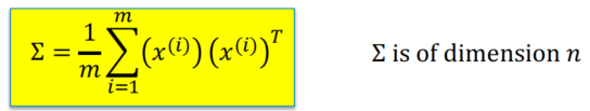
然后我们可以计算这个协方差矩阵${\sum }_{}$的特征值 $({\lambda }_i{)}_{i=1,....n}$。 我们保留前 $p$个最大的特征值
$({\lambda }_i{)}_{i=1,....p}$ 然后将数据投影到由 $p$ 个特征向量定义的$p$ 维空间中。这$p$ 个特征向量就叫作主成分(Principal Components).
PCA将数据变换到一个新的坐标系统，使得数据投影后的最大方差落在第一个坐标上（也叫第一主成分），第二大方差在第二个坐标上，依此类推

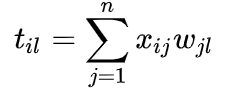
Mathematics of the PCA algorithm

如果 $X$ 是一个 $m\times n$ 的数据矩阵（ $m$ 个数据点， $n$个特征），每一个 $n$ 维的行向量 ${\left(x_{ij}\right)}_{j=1,2,..n}$ 映射到一个新的 $p$维向量 ${\left(t_{il}\right)}_{l=1,2,..p}$ ，这个新的向量就是${\left(x_{ij}\right)}_{j=1,2,..n}$的 $n$个坐标的线性组合：

我们希望向量${\left(t_{il}\right)}_{l=1,2,..p}$的范数最大化，或者第一个权重向量满足：

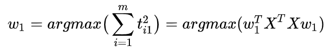
瑞利定理（Rayleigh Theorem）表明这个范数的最大值就是 $X^T$X 的最大特征值，也就是在 $w$ 是其对应特征值的情况下。

6. 变换步骤
   从上面两节我们可以看出，求样本 $x_i$ 的 $n^{{}^{\prime }}$ 维的主成分其实就是求样本集的协方差矩阵 $\frac{1}{m}X{X}^T$ 的前 $n^{{}^{\prime }}$ 个特征值对应特征向量矩阵 $P$，然后对于每个样本 $x_i$,做如下变换 $y_i=P{x}_i$ ，即达到降维的PCA目的。
   下面我们看看具体的算法流程：
   输入： n 维样本集 $X=(x_{1,....}{x}_m)$ ，要降维到的维数 $n^{{}^{\prime }}$
   输出：降维后的样本集 Y
   (1) 对所有的样本进行中心化 $x_i=x_i-\frac{1}{m}{\sum }_{j=1}^m{x}_j$
   (2) 第一步计算矩阵 X 的样本的协方差矩阵 S（此为不标准PCA，标准PCA计算相关系数矩阵C） $C=\frac{1}{m}X{X}^T$
   (3) 第二步计算协方差矩阵S（或C）的特征向量 e1,e2,…,eN和特征值 , t = 1,2,…,N
   (4) 将特征向量按对应特征值大小从上到下按行排列成矩阵，取前k行组成矩阵P
   (5) Y=PX即为降维到k维后的数据

3. 奇异值分解 – SVD

奇异值分解（Singular Value Decomposition）是线性代数中一种重要的矩阵分解，奇异值分解则是特征分解在任意矩阵上的推广。在信号处理、统计学等领域有重要应用。

4. 生成模型和GAN

Excercise

1 Calculate Logistic Regression by Hand

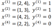
我们在平面上有四个点$x^{(i)}$，每个点的label $y^i$等于0或1。这四个点的points及其labels如下：

You are asked to perform the beginning of logistic regression by hand, using the notation from the slides that were presented during the course.
The logistic regression is based on a linear model with bias term combined with a sigmoid function. Therefore the linear function used is determined by three parameters (or weights):${\theta }_0$ 是bias. ${\theta }_1,{\theta }_2$ 分别是$x_1,x_2$的weight of $(x_1,x_2)$
我们要优化下面hypothesis function的weight

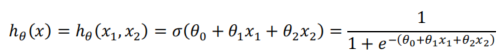
so that the labels of the four data points are properly approximated. 我们假设初始权重是随机抽样的，等于：$$({\theta }_0,{\theta }_1,{\theta }_2)=(0.9,1.3,0.1)$$
假设我们使用学习率 $\alpha$ 为0.1, 要求您手动计算, 第一次和第二次迭代后的更新权重$({\theta }_0,{\theta }_1,{\theta }_2)$

Answer

根据上面公式, 我们可以计算
$h_{\theta }(x^{(1)})=0.980$
$h_{\theta }(x^{(2)})=0.924$
$h_{\theta }(x^{(3)})=0.998$
$h_{\theta }(x^{(4)})=0.976$
Now calculate the cost function for each of the four points:
$$Cost(h_{\theta }(x^{(i)}),y^{(i)})=-y^{(i)}\log (h_{\theta }(x^{(i)}))-(1-y^{(i)})\log (1-(h_{\theta }(x^{(i)}))$$
we have
$Cost(h_{\theta }(x^{(1)}),y^{(1)})=0.020$
$Cost(h_{\theta }(x^{(2)}),y^{(2)})=0.079$
$Cost(h_{\theta }(x^{(3)}),y^{(3)})=6.302$
$Cost(h_{\theta }(x^{(4)}),y^{(4)})=3.724$
So the total initial cost function is the mean of the four above cost functions, that is:
$$J(\theta )=\frac{1}{m}{\sum }_{i=1}^{m}Cost(h_{\theta }(x^{(i)}),y^{(i)})$$
$J(\theta )=\frac{1}{4}\times [0.02+0.079+6.302+3.724]=2.531$
In order to update the three parameters $({\theta }_0,{\theta }_1,{\theta }_2)$, we now need to calculate the gradient of the cost function at each point $i$ in relation to each of the three parameters.
$$\frac{\partial J(\theta )}{\partial {\theta }_j}=\frac{1}{m}\sum _{i=1}^m[h_{\theta }(x^{(i)})-y^{(i)}]x_j^{(i)}$$
For a given point $x^{(i)}$, we have:
$\frac{\partial J(\theta )}{\partial {\theta }_0}=\frac{1}{m}{\sum }_{i=1}^m[h_{\theta }(x^{(i)})-y^{(i)}]x_0^{(i)}$
$\frac{\partial J(\theta )}{\partial {\theta }_1}=\frac{1}{m}{\sum }_{i=1}^m[h_{\theta }(x^{(i)})-y^{(i)}]x_1^{(i)}$
$\frac{\partial J(\theta )}{\partial {\theta }_2}=\frac{1}{m}{\sum }_{i=1}^m[h_{\theta }(x^{(i)})-y^{(i)}]x_2^{(i)}$
For point $x^{(1)}$
$\frac{\partial J(\theta )}{\partial {\theta }_0}=-0.020,\frac{\partial J(\theta )}{\partial {\theta }_1}=-0.040,\frac{\partial J(\theta )}{\partial {\theta }_2}=-0.079$
For point $x^{(2)}$
$\frac{\partial J(\theta )}{\partial {\theta }_0}=-0.076,\frac{\partial J(\theta )}{\partial {\theta }_1}=-0.076,\frac{\partial J(\theta )}{\partial {\theta }_2}=-0.228$
For point $x^{(3)}$
$\frac{\partial J(\theta )}{\partial {\theta }_0}=0.998,\frac{\partial J(\theta )}{\partial {\theta }_1}=3.993,\frac{\partial J(\theta )}{\partial {\theta }_2}=1.996$
For point $x^{(4)}$
$\frac{\partial J(\theta )}{\partial {\theta }_0}=0.976,\frac{\partial J(\theta )}{\partial {\theta }_1}=1.952,\frac{\partial J(\theta )}{\partial {\theta }_2}=1.952$
We add the gradients associated to each of the four data points, and we divide by the number of data points:
$\frac{\partial J(\theta )}{\partial {\theta }_0}=0.470,\frac{\partial J(\theta )}{\partial {\theta }_1}=1.457,\frac{\partial J(\theta )}{\partial {\theta }_2}=0.910$
Now that we have the gradients we can modify the parameters $({\theta }_0,{\theta }_1,{\theta }_2)$ using these gradients. If we denote $({\theta }_0^{{}^{\prime }},{\theta }_1^{{}^{\prime }},{\theta }_2^{{}^{\prime }})$:
$${\theta }_j^{{}^{\prime }}={\theta }_j-\alpha \frac{\partial J(\theta )}{\partial {\theta }_j}$$
If we use a value of 0.1 for the learning rate $\alpha$, we have:
${\theta }_0^{{}^{\prime }}=0.9-0.1\times 0.470=0.852$
${\theta }_1^{{}^{\prime }}=1.3-0.1\times 1.457=1.154$
${\theta }_2^{{}^{\prime }}=0.1-0.1\times 0.910=0.009$
Now let us start with the second iteration, starting this time with the values:
$({\theta }_0,{\theta }_1,{\theta }_2)=(0.852,1.154,0.009)$

2 Principal Components or Regression

该练习的目的是使用二维数据集，比较主成分分析（PCA）（一种无监督的学习方法）和线性回归（一种有监督的学习方法）。
可以从名为“House Prices：Advanced Regression Techniques”的Kaggle竞赛中获得使用的数据集。 它包含1460个训练数据点和80个features，这些features可能有助于预测房屋的售价。 该数据集在https://www.kaggle.com/c/houseprices-advanced-regression-techniques/data中有详细描述。 课程文件夹中也提供了名为houseprices.csv的数据集副本。

在本练习中，我们将重点关注文件houseprices.csv的以下两个变量：Saleprice：房屋售价（$）
GrLivArea：地面居住面积（square feet）我们将比较对这两个变量数据集应用regression或PCA的结果。 我们将使用变量名称 $x$ 表示GrLivArea，使用变量 $y$ 表示Saleprice. 以下是与数据集中的1460个房屋相关联的 $y$ vs $x$ 的cross-plot。
该练习关联了一个Python解决方案代码，称为PCARegression.py，并且可用

1. Problem 1

给出用于从$x$预测$y$的回归线的bias ${\theta }_0$和slope ${\theta }_1$“的数学表达式
计算回归参数${\theta }_0$和${\theta }_1$
Also calculate the regression parameters and the R2 variance score using the LinearRegression module in the sklearn.linear_model library. Check that your calculations of ${\theta }_0$ and ${\theta }_1$ are right.

Answer

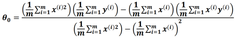
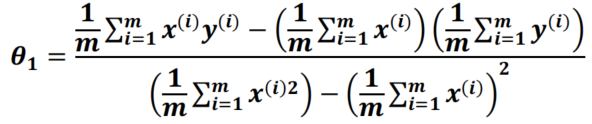
The formula for calculating ${\theta }_0$ and ${\theta }_1$ was given during this morning’s course:

"""
Calculate Regression lines, Orthogonal Regression line, and PCA on a 
two-dimensional dataset extracted from the Kaggle houseprices dataset.

Author: O. Dubrule
"""
import matplotlib.pyplot as plt
import pandas            as pd
import numpy             as np

from sklearn.linear_model  import LinearRegression
from sklearn.metrics       import r2_score
from sklearn.decomposition import PCA
from sklearn.preprocessing import StandardScaler


# Read and produce statistics on the two variables extracted from the Housprices dataset
houses = pd.read_csv('./Houseprices.csv')
print("houses ['SalePrice'] ")
print( houses ['SalePrice']  .describe())
print("houses ['GrLivArea'] ")
print( houses ['GrLivArea']  .describe())

# Create 1-D arrays for linear regression
x       =   houses[['GrLivArea']].values
y       =   houses[['SalePrice']].values

# Create and standardize 2-D array used for PCA and orthogonal regression
xy      =   houses[['GrLivArea','SalePrice']].values.astype(np.float)
sc      =   StandardScaler()
xy      =   sc.fit_transform(xy)
print('\n','Correlation Matrix after Standardization=',np.corrcoef(xy.transpose()))

def regression (U,V):
    """
    Calculate regression coefficients theta0 and theta1 for Linear Regression 
    of array V agains array U
    """ 
    U2        = np.multiply(U,U)
    V2        = np.multiply(V,V)
    UV        = np.multiply(U,V)
    
    Umean     = np.mean(U)
    Vmean     = np.mean(V)
    U2mean    = np.mean (U2)
    UVmean    = np.mean (UV)
    
    Theta0    = (U2mean*Vmean-Umean*UVmean)/(U2mean-Umean*Umean)
    Theta1    = (UVmean      -Umean*Vmean )/(U2mean-Umean*Umean)
    
    return Theta0,Theta1

def orthogonal_regression (U,V):   
    """
    The input parameters are the two centered arrays U and V respectively 
    containg the first and second coordinates of the data points
    """
    U2        = np.multiply(U,U)
    V2        = np.multiply(V,V)
    UV        = np.multiply(U,V)
    
    U2sum     = np.sum (U2)
    V2sum     = np.sum (V2)
    UVsum     = np.sum (UV)
    
    Term1     = V2sum-U2sum
    Term2     = Term1 * Term1
    Term3     = 4. * UVsum * UVsum
    Slope     = (Term1+np.sqrt(Term2+Term3))/(2.*UVsum)
   
    return Slope


# LINEAR REGRESSION: First we do y vs x
# First approach (analytical): calculate regression parameters using regression routine
Theta0 , Theta1  = regression(x,y)
Thetap0, Thetap1 = regression(y,x)
print('\n','REGRESSION:', '\n','Theta0     : %.4f'% Theta0 , 'Theta1     : %.4f'% Theta1 )
print(' Thetaprime0: %.4f'% Thetap0, '  Thetaprime1: %.4f'% Thetap1)

# Second approach (sklearn): first we do y vs x
regress  = LinearRegression(fit_intercept=True)
regress.fit (x, y)
y_       = regress.predict(x)
print('\n', 'Regression Coefficients for y vs x: \n', regress.intercept_, regress.coef_)
print(' R2 Variance score: %.2f' % r2_score(y, y_))

# Second approach (sklearn): now  we do x vs y
regress.fit (y, x)
x_     = regress.predict (y)
print('\n', 'Regression Coefficients for x vs y: \n', regress.intercept_, regress.coef_)
print(' R2 Variance score: %.2f' % r2_score(x,x_))

# PCA:
# First approach (analytical): calculate slope of line using orthogonal_regression routine
slope_ortho = orthogonal_regression(xy[:,0],xy[:,1])

# Second approach:  use sklearn's PCA to calculate slope of major axis
pca    = PCA (n_components=1)
pca.fit  (xy) 
print    ('\n'*1, 'PCA:','\n'*1,'Explained Variance:', pca.explained_variance_ratio_)
print    ('Coordinates in Feature Space of the PCA Component:','\n',pca.components_)

# Calculate slope of PCA line and compare with slope of orthogonal regression
slope_pca = pca.components_[0,1]/pca.components_[0,0]
print (' Slope from PCA:', slope_pca, ' Slope from orthogonal regression: ', slope_ortho)

# Now plot all the results
plt.figure  (figsize=(10, 8))

# Plot the input data in red
plt.scatter (x, y, s=20, color='red')

# Plot the two Regression Lines (y vs x and x vs y) in blue and black
plt.plot    (x  , y_ , color='blue'   ,linewidth=3, label='Regression y vs x')
plt.plot    (x_ , y  , color='black'  ,linewidth=3, label='Regression x vs y')
"""
Correct for the slopes for plotting, because of the initial scaling of the input data
"""
stddev      = np.sqrt(sc.var_)
slope_ortho = slope_ortho * stddev[1]/stddev[0]
slope_pca   = slope_pca   * stddev[1]/stddev[0]
"""
Plot PCA and Orthogonal Regression lines, which should overlap (we should only see the green
line as it is the  second one to be plotted)
"""
plt.plot    (x,((np.mean(y) - slope_pca  *np.mean(x)) + slope_pca  *x), color='cyan'    ,linewidth=3)
plt.plot    (x,((np.mean(y) - slope_ortho*np.mean(x)) + slope_ortho*x), color='green'   ,linewidth=3, label= 'PCA (or Othogonal Regression)')

plt.xlim(0.,6000.)
plt.ylim(0.,800000.)

plt.xlabel('Greater Living Area Above Ground')
plt.ylabel('House Sale Price')

plt.title ('Houses Sale Price: Compare Linear Regressions, Orthogonal Regression and PCA')

plt.legend()
plt.show()

/*
houses ['SalePrice'] 
count      1460.000000
mean     180921.195890
std       79442.502883
min       34900.000000
25%      129975.000000
50%      163000.000000
75%      214000.000000
max      755000.000000
Name: SalePrice, dtype: float64
houses ['GrLivArea']
count    1460.000000
mean     1515.463699
std       525.480383
min       334.000000
25%      1129.500000
50%      1464.000000
75%      1776.750000
max      5642.000000
Name: GrLivArea, dtype: float64

 Correlation Matrix after Standardization= [[1.         0.70862448]
 [0.70862448 1.        ]]

 REGRESSION:
 Theta0     : 18569.0259 Theta1     : 107.1304
 Thetaprime0: 667.4377   Thetaprime1: 0.0047

 Regression Coefficients for y vs x:
 [18569.02585649] [[107.13035897]]
 R2 Variance score: 0.50

 Regression Coefficients for x vs y:
 [667.43765635] [[0.00468727]]
 R2 Variance score: 0.50

 PCA:
 Explained Variance: [0.85431224]
Coordinates in Feature Space of the PCA Component:
 [[0.70710678 0.70710678]]
 Slope from PCA: 1.0000000000000002  Slope from orthogonal regression:  0.9999999999999998
*/

运行上面程序得出:
${\theta }_0$=18569.0259 and ${\theta }_1$= 107.1304
Using the sklearn LinearRegression module gives us the same values for both parameters and a value for the R2 variance score equal to 0.50, which indicates a correlation coefficient of $\rho =\sqrt{0.5}=0.71$

2. Problem 2

给出用于从$y$预测$x$的回归线的偏差项${\theta }_0^{{}^{\prime }}$和斜率${\theta }_1^{{}^{\prime }}$的数学表达式
与上面公式相似,只是需要调换$x,y$的顺序

根据给出的代码, 我们可以得出
$${\theta }_0^{{}^{\prime }}=667.4377,{\theta }_1^{{}^{\prime }}=0.0047$$
与上面一样, R2 variance socre of 0.5. 因为we saw above that the R2 variance score is equal to the square of the correlation coefficient, which is the same for $y$ vs $x$ or $x$ vs $y$

3. Problem 3

Plot the two regression lines calculated in the previous questions, and cross-plot the dataset on the same figure.

We observe that the two lines intersect at the mean of both variables.
一个有趣的特性是the product of the slopes of the two lines is equal to the square of the correlation coefficient, which is also the R2 variance score:
$$107.1304\times 0.0047=0.50$$

4. Problem 4

With regression, as seen in the two previous questions, what is minimized is the sum of squares of the differences between the data values and the regression lines.这可以在下面的图片中进行总结(the sum of the squares of the red lines are minimized by regression of $y$ vs $x$, the sum of the squares of the green lines are minimized by regression of $x$ vs $y$). 另一方面，PCA最小化橙色线的平方和，即与计算出的主轴垂直的线的平方和 (PCA maximizes the variance of the data projected on the principal axis).

There are two ways to calculate the slope of the PCA line in two dimensions(计算斜率就足够了，因为第二个参数可以从以下事实得出：与两条回归线一样，PCA线会经过与两个变量的平均值相关的点)
The first approach is to calculate it analytically using the method known as Orthogonal Regression, where the sum of the squares of the orange segments in the above figure is minimized.It can be demonstrated that the formula for the slope is:

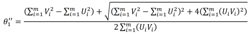
Where $U$ and $V$ are the centered variables $x$ and $y$, that is the variables $x$ and $y$ after substraction of their mean:
$U=x-m_x,V=y-m_y$
The second approach is to calculate it using the PCA module in the sklearn.decomposition library. 使用第二种方法，it is important to first standardize Saleprice and GrLivArea.使用两种方法并验证您获得相同的结果。
Using either the equation given above for ${\theta }_1^{{}^{\prime \prime }}$, or the sklearn PCA module, we obtain the same result:
$${\theta }_1^{{}^{\prime \prime }}=1$$

5. Problem 5

Compare the three lines on the same cross-plot. What do you observe?

我们观察到PCA线正好位于两个先前计算的回归线之间。This is expected as, in the PCA formalism, x and y play a symmetric role.如前所述，PCA（或正交回归）是一种不受监督的技术：该算法在平面中以一组点表示，and it has to project this set on points on the line that loses a minimum amount of information after the points have been projected on the line.
另一方面，通过回归，the algorithm is given either a set of x values labelled by y or a set of y values labelled by x.
代码PCARegression.py提供了上述问题的解决方案