Python数据分析实战【十一】：学习用scorecardpy搭建风控评分卡模型【文末源码地址】

评分卡模型

• scorecardpy库

github地址：https://github.com/ShichenXie/scorecardpy

一、数据预处理

import scorecardpy as sc
import pandas as pd
import numpy as np

scorecardpy自带数据

dat = sc.germancredit()

查看数据行列

dat.shape
(1000, 21)

数据是由1000行，21列数据组成

查看数据内容,用sample()比head()可以看更多的数据

dat.sample(5)

	status.of.existing.checking.account	duration.in.month	credit.history	purpose	credit.amount	savings.account.and.bonds	present.employment.since	installment.rate.in.percentage.of.disposable.income	personal.status.and.sex	other.debtors.or.guarantors	...	property	age.in.years	other.installment.plans	housing	number.of.existing.credits.at.this.bank	job	number.of.people.being.liable.to.provide.maintenance.for	telephone	foreign.worker	creditability
547	no checking account	24	existing credits paid back duly till now	radio/television	1552	... < 100 DM	4 <= ... < 7 years	3	male : single	none	...	car or other, not in attribute Savings account...	32	bank	own	1	skilled employee / official	2	none	yes	good
617	... < 0 DM	6	critical account/ other credits existing (not ...	car (new)	3676	... < 100 DM	1 <= ... < 4 years	1	male : single	none	...	real estate	37	none	rent	3	skilled employee / official	2	none	yes	good
186	0 <= ... < 200 DM	9	all credits at this bank paid back duly	car (used)	5129	... < 100 DM	... >= 7 years	2	female : divorced/separated/married	none	...	unknown / no property	74	bank	for free	1	management/ self-employed/ highly qualified em...	2	yes, registered under the customers name	yes	bad
776	no checking account	36	critical account/ other credits existing (not ...	car (new)	3535	... < 100 DM	4 <= ... < 7 years	4	male : single	none	...	car or other, not in attribute Savings account...	37	none	own	2	skilled employee / official	1	yes, registered under the customers name	yes	good
243	no checking account	12	critical account/ other credits existing (not ...	business	1185	... < 100 DM	1 <= ... < 4 years	3	female : divorced/separated/married	none	...	real estate	27	none	own	2	skilled employee / official	1	none	yes	good

5 rows × 21 columns

可以发现有none出现，代表的是缺失，可以用np.nan替换，方便统计每一个变量的缺失占比情况

dat = dat.replace('none',np.nan)

统计每个变量的缺失占比情况

(dat.isnull().sum()/dat.shape[0]).map(lambda x:"{:.2%}".format(x))

status.of.existing.checking.account                          0.00%
duration.in.month                                            0.00%
credit.history                                               0.00%
purpose                                                      0.00%
credit.amount                                                0.00%
savings.account.and.bonds                                    0.00%
present.employment.since                                     0.00%
installment.rate.in.percentage.of.disposable.income          0.00%
personal.status.and.sex                                      0.00%
other.debtors.or.guarantors                                 90.70%
present.residence.since                                      0.00%
property                                                     0.00%
age.in.years                                                 0.00%
other.installment.plans                                     81.40%
housing                                                      0.00%
number.of.existing.credits.at.this.bank                      0.00%
job                                                          0.00%
number.of.people.being.liable.to.provide.maintenance.for     0.00%
telephone                                                   59.60%
foreign.worker                                               0.00%
creditability                                                0.00%
dtype: object

other.debtors.or.guarantors（担保人）这一列数据的缺失占比超过90%，可以删除。

other.installment.plans（分期付款计划）这一列缺失占比也较高，只有两个分类，也可以删除。

dat["other.installment.plans"].value_counts()

bank      139
stores     47
Name: other.installment.plans, dtype: int64

telephone（电话）对建模没有太大意义，就像姓名，对建模没有太大影响。但是电话是否填写应该被考虑进去，这里先不讨论。

dat = dat.drop(columns=["other.debtors.or.guarantors","other.installment.plans","telephone"])

查看数据的信息

dat.info()

<class 'pandas.core.frame.DataFrame'>
RangeIndex: 1000 entries, 0 to 999
Data columns (total 18 columns):
 #   Column                                                    Non-Null Count  Dtype   
---  ------                                                    --------------  -----   
 0   status.of.existing.checking.account                       1000 non-null   category
 1   duration.in.month                                         1000 non-null   int64   
 2   credit.history                                            1000 non-null   category
 3   purpose                                                   1000 non-null   object  
 4   credit.amount                                             1000 non-null   int64   
 5   savings.account.and.bonds                                 1000 non-null   category
 6   present.employment.since                                  1000 non-null   category
 7   installment.rate.in.percentage.of.disposable.income       1000 non-null   int64   
 8   personal.status.and.sex                                   1000 non-null   category
 9   present.residence.since                                   1000 non-null   int64   
 10  property                                                  1000 non-null   category
 11  age.in.years                                              1000 non-null   int64   
 12  housing                                                   1000 non-null   category
 13  number.of.existing.credits.at.this.bank                   1000 non-null   int64   
 14  job                                                       1000 non-null   category
 15  number.of.people.being.liable.to.provide.maintenance.for  1000 non-null   int64   
 16  foreign.worker                                            1000 non-null   category
 17  creditability                                             1000 non-null   object  
dtypes: category(9), int64(7), object(2)
memory usage: 80.8+ KB

可以看出数据是由int64，category，object类型的数据组成，category类型的数据在pandas中很特殊，建议转为object类型数据。

查看每个变量有多少分类

# 顺便把category类型的数据转为object
for c in dat.columns:
    if str(dat[c].dtype) == "category":
        dat[c] = dat[c].astype(str)
    print(c,"：",len(dat[c].unique()))

status.of.existing.checking.account ： 4
duration.in.month ： 33
credit.history ： 5
purpose ： 10
credit.amount ： 921
savings.account.and.bonds ： 5
present.employment.since ： 5
installment.rate.in.percentage.of.disposable.income ： 4
personal.status.and.sex ： 3
present.residence.since ： 4
property ： 4
age.in.years ： 53
housing ： 3
number.of.existing.credits.at.this.bank ： 4
job ： 4
number.of.people.being.liable.to.provide.maintenance.for ： 2
foreign.worker ： 2
creditability ： 2

可以看到credit.amount（金额）有921个不同的类别，age.in.years（年龄）有53个类别。
类别较多的需要合并区间，类别少的视情况而定。

描述性统计

查看每一个变量的均值，最大，最小，分位数

dat.describe()

	duration.in.month	credit.amount	installment.rate.in.percentage.of.disposable.income	present.residence.since	age.in.years	number.of.existing.credits.at.this.bank	number.of.people.being.liable.to.provide.maintenance.for
count	1000.000000	1000.000000	1000.000000	1000.000000	1000.000000	1000.000000	1000.000000
mean	20.903000	3271.258000	2.973000	2.845000	35.546000	1.407000	1.155000
std	12.058814	2822.736876	1.118715	1.103718	11.375469	0.577654	0.362086
min	4.000000	250.000000	1.000000	1.000000	19.000000	1.000000	1.000000
25%	12.000000	1365.500000	2.000000	2.000000	27.000000	1.000000	1.000000
50%	18.000000	2319.500000	3.000000	3.000000	33.000000	1.000000	1.000000
75%	24.000000	3972.250000	4.000000	4.000000	42.000000	2.000000	1.000000
max	72.000000	18424.000000	4.000000	4.000000	75.000000	4.000000	2.000000

数据之间的相关性

dat.corr()

	duration.in.month	credit.amount	installment.rate.in.percentage.of.disposable.income	present.residence.since	age.in.years	number.of.existing.credits.at.this.bank	number.of.people.being.liable.to.provide.maintenance.for
duration.in.month	1.000000	0.624984	0.074749	0.034067	-0.036136	-0.011284	-0.023834
credit.amount	0.624984	1.000000	-0.271316	0.028926	0.032716	0.020795	0.017142
installment.rate.in.percentage.of.disposable.income	0.074749	-0.271316	1.000000	0.049302	0.058266	0.021669	-0.071207
present.residence.since	0.034067	0.028926	0.049302	1.000000	0.266419	0.089625	0.042643
age.in.years	-0.036136	0.032716	0.058266	0.266419	1.000000	0.149254	0.118201
number.of.existing.credits.at.this.bank	-0.011284	0.020795	0.021669	0.089625	0.149254	1.000000	0.109667
number.of.people.being.liable.to.provide.maintenance.for	-0.023834	0.017142	-0.071207	0.042643	0.118201	0.109667	1.000000

可以看出，credit.amount与duration.in.month的相关性为0.624984。可以根据实际业务，将相关性高的变量保留一个。

二、数据筛选

参考文章：https://zhuanlan.zhihu.com/p/80134853

评分卡建模常用WOE、IV来筛选变量，通常选择IV值>0.02的变量。IV值越大，变量对y的预测能力较强，就越应该进入模型中。

WOE：(Weight of Evidence)中文“证据权重”，某个变量的区间对y的影响程度。

• 计算方法：
  $$WO{E}_i=ln(\frac{R_{0i}}{R_{0T}})-ln(\frac{R_{1i}}{R_{1T}})$$
  $$\begin{gathered} R_{0i}：变量的第i个区间，y=0的个数。 \\ {R}_{0T}：y=0的个数。 \\ {R}_{1i}：变量的第i个区间，y=1的个数。 \\ {R}_{1T}：y=1的个数。 \end{gathered}$$

• 举例说明：
  将age.in.years划分为[-inf,26.0),[26.0,35.0),[35.0,40.0),[40.0,inf)四个区间，统计各个区间y=0(good)，y=1(bad)的数量，计算WOE。
  比如计算age.in.year在[26,35)区间的WOE：
  $$WO{E}_i=ln(\frac{R_{0i}}{R_{0T}})-ln(\frac{R_{1i}}{R_{1T}})=ln(\frac{246}{700})-ln(\frac{112}{300})=-0.060465$$
  同理可以计算出其他区间对应的WOE值。

IV:（Information Value）中文“信息价值”，变量所含信息的价值。

• 计算方法：
  $$IV=\sum _{i=1}^n(\frac{R_{0i}}{R_{0T}}-\frac{R_{1i}}{R_{1T}})\ast WO{E}_i$$
• 举例说明：
  $$\begin{gathered} IV=\sum _{i=1}^n(\frac{R_{0i}}{R_{0T}}-\frac{R_{1i}}{R_{1T}})\ast WO{E}_i \\ =(\frac{110}{700}-\frac{80}{300})\ast 0.528844 \\ +(\frac{246}{700}-\frac{112}{300})\ast 0.060465 \\ +(\frac{123}{700}-\frac{30}{300})\ast -0.563689 \\ +(\frac{221}{700}-\frac{78}{300})\ast -0.194156 \\ =0.112742 \end{gathered}$$

公式看似复杂，其实仔细想想，用到的知识也不是很难。另外，这些程序scorecardpy中已经实现，只需要调用传参即可。

用scorecardpy计算的age.in.years的WOE：

# bins_adj_df[bins_adj_df.variable=="age.in.years"]

	level_1	variable	bin	count	count_distr	good	bad	badprob	woe	bin_iv	total_iv	breaks	is_special_values
4	0	age.in.years	[-inf,26.0)	190	0.190	110	80	0.421053	0.528844	0.057921	0.112742	26.0	False
5	1	age.in.years	[26.0,35.0)	358	0.358	246	112	0.312849	0.060465	0.001324	0.112742	35.0	False
6	2	age.in.years	[35.0,40.0)	153	0.153	123	30	0.196078	-0.563689	0.042679	0.112742	40.0	False
7	3	age.in.years	[40.0,inf)	299	0.299	221	78	0.260870	-0.194156	0.010817	0.112742	inf	False

sc.var_filter()

• dt：数据
• y：y变量名
• iv_limit：0.02
• missing_limit：0.95
• identical_limit：0.95
• positive：坏样本的标签
• dt：DataFrame数据
• var_rm：强制删除变量的名称
• var_kp：强制保留变量的名称
• return_rm_reason：是否返回每个变量被删除的原因

dt_s = sc.var_filter(dat,y="creditability",iv_limit=0.02)

dat.shape

(1000, 18)

dt_s.shape

(1000, 13)

可以看出，用var_filter()方法，将变量从18个筛选到13个变量。

划分数据

sc.split_df(dt, y=None, ratio=0.7, seed=186)

train,test = sc.split_df(dt=dt_s,y="creditability").values()

训练数据y的统计：

train.creditability.value_counts()

0    490
1    210
Name: creditability, dtype: int64

测试数据y的统计：

test.creditability.value_counts()

0    210
1     90
Name: creditability, dtype: int64

三、 变量分箱

常用的分箱：卡方分箱，决策树分箱… ，这里简单介绍一下卡方分箱。

为什么要分箱？
分箱之后，变量的轻微波动，不影响模型的稳定。比如：收入这一变量，10000和11000对y的影响可能是一样的，将其归为一类是一个不错的选择。

分箱要求？

1. 变量的类别在5到7类最好
2. 有序，单调，平衡

卡方分箱：

参考文章：https://zhuanlan.zhihu.com/p/115267395

• 卡方分箱的思想，衡量预测值与观察值的差异，究竟有多大的概率是由随机因素引起的。
• 卡方值计算：
  $${\chi }^2=\sum _{i=1}^n\sum _{c=1}^m\frac{(A_{ic}-E_{ic}{)}^2}{E_{ic}}$$
  $$\begin{gathered} n：划分的区间总数。 \\ m：y的类别，一般为2个。 \\ {A}_{ic}：实际样本在每个区间统计的数量。 \end{gathered}$$

$$E_{ic}：期望样本在每个区间的数量，E_{ic}=\frac{T_i\ast T_c}{T}，T_i：第i个分组的总数，T_c：第c个类别的总数，T：总样本数。$$

• 步骤：（数值型数据）
  1. 将数据去重并排序，得到A1，A2，A3等分组区间，统计每个区间的量。
  2. 计算A1与A2的卡方值，计算A2与A3的卡方值，（计算相邻区间的卡方值）
  3. 如果相邻的卡方值小于阈值（根据自由度和置信度计算得出的出的阈值），就合并区间为一个新的区间。
  4. 重复第2、3步的操作。直到达到某个条件停止计算。
  5. 当最小的卡方值大于阈值，停止。
  6. 当划分的区间到达指定的区间个数，停止。

woebin()

• scorecardpy默认使用决策树分箱，method=‘tree’
• 这里使用卡方分箱，method=‘chimerge’
• 返回的是一个字典数据，用pandas.concat()查看所有数据

bins = sc.woebin(dt_s,y="creditability",method="chimerge")

bins["installment.rate.in.percentage.of.disposable.income"]

	variable	bin	count	count_distr	good	bad	badprob	woe	bin_iv	total_iv	breaks	is_special_values
0	installment.rate.in.percentage.of.disposable.i...	[-inf,3.0)	367	0.367	271	96	0.261580	-0.190473	0.012789	0.019769	3.0	False
1	installment.rate.in.percentage.of.disposable.i...	[3.0,inf)	633	0.633	429	204	0.322275	0.103961	0.006980	0.019769	inf	False

bins_df = pd.concat(bins).reset_index().drop(columns="level_0")

bins_df

	level_1	variable	bin	count	count_distr	good	bad	badprob	woe	bin_iv	total_iv	breaks	is_special_values
0	0	credit.amount	[-inf,1400.0)	267	0.267	185	82	0.307116	0.033661	0.000305	0.171431	1400.0	False
1	1	credit.amount	[1400.0,1800.0)	105	0.105	87	18	0.171429	-0.728239	0.046815	0.171431	1800.0	False
2	2	credit.amount	[1800.0,2000.0)	60	0.060	39	21	0.350000	0.228259	0.003261	0.171431	2000.0	False
3	3	credit.amount	[2000.0,4000.0)	322	0.322	248	74	0.229814	-0.362066	0.038965	0.171431	4000.0	False
4	4	credit.amount	[4000.0,inf)	246	0.246	141	105	0.426829	0.552498	0.082085	0.171431	inf	False
5	0	age.in.years	[-inf,26.0)	190	0.190	110	80	0.421053	0.528844	0.057921	0.123935	26.0	False
6	1	age.in.years	[26.0,35.0)	358	0.358	246	112	0.312849	0.060465	0.001324	0.123935	35.0	False
7	2	age.in.years	[35.0,37.0)	79	0.079	67	12	0.151899	-0.872488	0.048610	0.123935	37.0	False
8	3	age.in.years	[37.0,inf)	373	0.373	277	96	0.257373	-0.212371	0.016080	0.123935	inf	False
9	0	housing	own	713	0.713	527	186	0.260870	-0.194156	0.025795	0.082951	own	False
10	1	housing	rent%,%for free	287	0.287	173	114	0.397213	0.430205	0.057156	0.082951	rent%,%for free	False
11	0	property	real estate	282	0.282	222	60	0.212766	-0.461035	0.054007	0.112634	real estate	False
12	1	property	building society savings agreement/ life insur...	564	0.564	391	173	0.306738	0.031882	0.000577	0.112634	building society savings agreement/ life insur...	False
13	2	property	unknown / no property	154	0.154	87	67	0.435065	0.586082	0.058050	0.112634	unknown / no property	False
14	0	duration.in.month	[-inf,8.0)	87	0.087	78	9	0.103448	-1.312186	0.106849	0.282618	8.0	False
15	1	duration.in.month	[8.0,16.0)	344	0.344	264	80	0.232558	-0.346625	0.038294	0.282618	16.0	False
16	2	duration.in.month	[16.0,34.0)	399	0.399	270	129	0.323308	0.108688	0.004813	0.282618	34.0	False
17	3	duration.in.month	[34.0,44.0)	100	0.100	58	42	0.420000	0.524524	0.029973	0.282618	44.0	False
18	4	duration.in.month	[44.0,inf)	70	0.070	30	40	0.571429	1.134980	0.102689	0.282618	inf	False
19	0	status.of.existing.checking.account	no checking account	394	0.394	348	46	0.116751	-1.176263	0.404410	0.666012	no checking account	False
20	1	status.of.existing.checking.account	... >= 200 DM / salary assignments for at leas...	63	0.063	49	14	0.222222	-0.405465	0.009461	0.666012	... >= 200 DM / salary assignments for at leas...	False
21	2	status.of.existing.checking.account	0 <= ... < 200 DM	269	0.269	164	105	0.390335	0.401392	0.046447	0.666012	0 <= ... < 200 DM	False
22	3	status.of.existing.checking.account	... < 0 DM	274	0.274	139	135	0.492701	0.818099	0.205693	0.666012	... < 0 DM	False
23	0	installment.rate.in.percentage.of.disposable.i...	[-inf,3.0)	367	0.367	271	96	0.261580	-0.190473	0.012789	0.019769	3.0	False
24	1	installment.rate.in.percentage.of.disposable.i...	[3.0,inf)	633	0.633	429	204	0.322275	0.103961	0.006980	0.019769	inf	False
25	0	savings.account.and.bonds	... >= 1000 DM%,%500 <= ... < 1000 DM%,%unknow...	294	0.294	245	49	0.166667	-0.762140	0.142266	0.189391	... >= 1000 DM%,%500 <= ... < 1000 DM%,%unknow...	False
26	1	savings.account.and.bonds	100 <= ... < 500 DM%,%... < 100 DM	706	0.706	455	251	0.355524	0.252453	0.047125	0.189391	100 <= ... < 500 DM%,%... < 100 DM	False
27	0	present.employment.since	4 <= ... < 7 years%,%... >= 7 years	427	0.427	324	103	0.241218	-0.298717	0.035704	0.082865	4 <= ... < 7 years%,%... >= 7 years	False
28	1	present.employment.since	1 <= ... < 4 years	339	0.339	235	104	0.306785	0.032103	0.000352	0.082865	1 <= ... < 4 years	False
29	2	present.employment.since	unemployed%,%... < 1 year	234	0.234	141	93	0.397436	0.431137	0.046809	0.082865	unemployed%,%... < 1 year	False
30	0	personal.status.and.sex	male : single%,%male : married/widowed	640	0.640	469	171	0.267188	-0.161641	0.016164	0.042633	male : single%,%male : married/widowed	False
31	1	personal.status.and.sex	female : divorced/separated/married	360	0.360	231	129	0.358333	0.264693	0.026469	0.042633	female : divorced/separated/married	False
32	0	credit.history	critical account/ other credits existing (not ...	293	0.293	243	50	0.170648	-0.733741	0.132423	0.291829	critical account/ other credits existing (not ...	False
33	1	credit.history	delay in paying off in the past%,%existing cre...	618	0.618	421	197	0.318770	0.087869	0.004854	0.291829	delay in paying off in the past%,%existing cre...	False
34	2	credit.history	all credits at this bank paid back duly%,%no c...	89	0.089	36	53	0.595506	1.234071	0.154553	0.291829	all credits at this bank paid back duly%,%no c...	False
35	0	purpose	retraining%,%car (used)%,%radio/television	392	0.392	312	80	0.204082	-0.513679	0.091973	0.142092	retraining%,%car (used)%,%radio/television	False
36	1	purpose	furniture/equipment%,%domestic appliances%,%bu...	608	0.608	388	220	0.361842	0.279920	0.050119	0.142092	furniture/equipment%,%domestic appliances%,%bu...	False

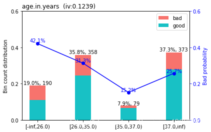
woebin_plot()

• 制作变量分布图

bins["age.in.years"]

	variable	bin	count	count_distr	good	bad	badprob	woe	bin_iv	total_iv	breaks	is_special_values
0	age.in.years	[-inf,26.0)	190	0.190	110	80	0.421053	0.528844	0.057921	0.123935	26.0	False
1	age.in.years	[26.0,35.0)	358	0.358	246	112	0.312849	0.060465	0.001324	0.123935	35.0	False
2	age.in.years	[35.0,37.0)	79	0.079	67	12	0.151899	-0.872488	0.048610	0.123935	37.0	False
3	age.in.years	[37.0,inf)	373	0.373	277	96	0.257373	-0.212371	0.016080	0.123935	inf	False

sc.woebin_plot(bins["age.in.years"])

sc.woebin_plot(bins["credit.amount"])

​

从变量的分布图，看出bad_prob、credit.amount这两个变量并不单调，接下来就需要调整一下区间。

分箱调整

• scorecardpy可以自定义分箱，也可以自动分箱。
• 自己手动调整比较好（根据业务，实际经验调整）

# 自动分箱
# break_adj = sc.woebin_adj(dt_s,y="creditability",bins=bins)

bins["credit.amount"]

	variable	bin	count	count_distr	good	bad	badprob	woe	bin_iv	total_iv	breaks	is_special_values
0	credit.amount	[-inf,1400.0)	267	0.267	185	82	0.307116	0.033661	0.000305	0.171431	1400.0	False
1	credit.amount	[1400.0,1800.0)	105	0.105	87	18	0.171429	-0.728239	0.046815	0.171431	1800.0	False
2	credit.amount	[1800.0,2000.0)	60	0.060	39	21	0.350000	0.228259	0.003261	0.171431	2000.0	False
3	credit.amount	[2000.0,4000.0)	322	0.322	248	74	0.229814	-0.362066	0.038965	0.171431	4000.0	False
4	credit.amount	[4000.0,inf)	246	0.246	141	105	0.426829	0.552498	0.082085	0.171431	inf	False

将年龄划分在[-inf,26.0)，[26.0,35.0)，[35.0,40.0)，[40.0,inf)区间大致能满足单调性。 金额划分在[-inf,1400.0)，[1400.0,1900.0)，[1900.0,4000.0)，[4000.0,inf)区间大致能满足单调性。

# 手动分箱
break_adj = {
    'age.in.years':[26,35,40],
    'credit.amount':[1400,1900,4000]
}
bins_adj = sc.woebin(dt_s,y="creditability",breaks_list=break_adj)

bins_adj_df = pd.concat(bins_adj).reset_index().drop(columns="level_0")

bins_adj_df[bins_adj_df.variable.isin(["age.in.years",'credit.amount'])]

	level_1	variable	bin	count	count_distr	good	bad	badprob	woe	bin_iv	total_iv	breaks	is_special_values
0	0	credit.amount	[-inf,1400.0)	267	0.267	185	82	0.307116	0.033661	0.000305	0.141144	1400.0	False
1	1	credit.amount	[1400.0,1900.0)	131	0.131	104	27	0.206107	-0.501256	0.029359	0.141144	1900.0	False
2	2	credit.amount	[1900.0,4000.0)	356	0.356	270	86	0.241573	-0.296777	0.029395	0.141144	4000.0	False
3	3	credit.amount	[4000.0,inf)	246	0.246	141	105	0.426829	0.552498	0.082085	0.141144	inf	False
4	0	age.in.years	[-inf,26.0)	190	0.190	110	80	0.421053	0.528844	0.057921	0.112742	26.0	False
5	1	age.in.years	[26.0,35.0)	358	0.358	246	112	0.312849	0.060465	0.001324	0.112742	35.0	False
6	2	age.in.years	[35.0,40.0)	153	0.153	123	30	0.196078	-0.563689	0.042679	0.112742	40.0	False
7	3	age.in.years	[40.0,inf)	299	0.299	221	78	0.260870	-0.194156	0.010817	0.112742	inf	False

sc.woebin_plot(bins_adj["age.in.years"])

sc.woebin_plot(bins_adj['credit.amount']

四、WOE转化

将原始数据都转化为对应区间的WOE值，当然也可以不转化，但是转化之后：

• 变量内部之间可以比较
• 变量与变量之间也可以比较
• 所有变量都在同一“维度”下

train_woe = sc.woebin_ply(train,bins_adj)

test_woe = sc.woebin_ply(test,bins_adj)

train_woe.sample(5)

	creditability	credit.amount_woe	age.in.years_woe	housing_woe	property_woe	duration.in.month_woe	status.of.existing.checking.account_woe	installment.rate.in.percentage.of.disposable.income_woe	savings.account.and.bonds_woe	present.employment.since_woe	personal.status.and.sex_woe	credit.history_woe	purpose_woe
723	0	0.033661	-0.194156	-0.194156	-0.461035	-0.346625	0.614204	0.103961	-0.762140	0.032103	0.264693	0.088319	-0.410063
331	1	-0.501256	0.060465	-0.194156	-0.461035	0.108688	-1.176263	0.103961	0.139552	0.032103	0.264693	-0.733741	0.279920
690	0	0.033661	0.528844	-0.194156	0.028573	-0.346625	0.614204	-0.155466	0.271358	0.032103	0.264693	-0.733741	0.279920
537	0	-0.296777	-0.563689	-0.194156	0.028573	0.108688	0.614204	0.103961	0.271358	-0.235566	0.264693	-0.733741	0.279920
0	0	0.033661	-0.194156	-0.194156	-0.461035	-1.312186	0.614204	0.103961	-0.762140	-0.235566	-0.165548	-0.733741	-0.410063

五、建立模型

逻辑回归，挺复杂的。

from sklearn.linear_model import LogisticRegression

y_train = train_woe.loc[:,"creditability"]
X_train = train_woe.loc[:,train_woe.columns!="creditability"]

y_test = test_woe.loc[:,"creditability"]
X_test = test_woe.loc[:,test_woe.columns!="creditability"]

lr = LogisticRegression(penalty='l1',C=0.9,solver='saga',n_jobs=-1)
lr.fit(X_train,y_train)

LogisticRegression(C=0.9, n_jobs=-1, penalty='l1', solver='saga')

lr.coef_

array([[0.77881419, 0.6892819 , 0.36660545, 0.37598509, 0.59990642,
        0.75916199, 1.68181704, 0.50153176, 0.23641609, 0.70438936,
        0.63125597, 0.99437898]])

lr.intercept_

array([-0.82463787])

六、模型评估

逻辑回归，预测结果为接近1的概率值。
0.6表示：数据划分为标签1的概率为0.6。那么究竟多大的概率才能划为标签1呢？这就需要一个阈值。这个阈值可以根据KS的值来确定。高于阈值得划分为1标签，低于阈值得划分为0标签。

TRP与FRP：
$$TRP=\frac{预测为1，真实值为1的数据量}{预测为1的总量}$$
$$FRP=\frac{预测为0，真实值为1的数据量}{预测为0的总量}$$
ROC曲线绘制步骤：

1. 将预测的y_score去重排序后得到一系列阈值。
2. 用每一个y_score做为阈值，统计数量并计算TRP、FRP的值。
3. 这样得到一组数据后，以FPR为横坐标，TPR为纵轴标绘制图像。

AUC：

• ROC曲线与横坐标轴围成的面积。

KS曲线：用来确定最好的阈值
$$KS=max(TRP-FRP)$$

• x轴为一些阈值的长度（区间序号都行），将TRP、FRP绘制在同一个坐标轴中。

train_pred = lr.predict_proba(X_train)[:,1]
test_pred =  lr.predict_proba(X_test)[:,1]

train_perf = sc.perf_eva(y_train,train_pred,title="train")

test_perf = sc.perf_eva(y_test,test_pred,title="test")

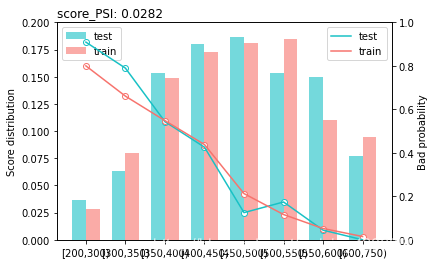
七、评分稳定性

PSI（Population Stability Index）群组稳定性指标

• 模型在训练数据得到的实际分布(A)，与测试集上得到的预期分布(E)
  $$PSI=\sum _{i=1}^n(A_i-E_i)\ast ln(\frac{A_i}{E_i})$$
  $$A_i：实际分布在第i个区间的数量。$$

$$E_i：预期分布在第i个区间的数量。$$

PSI越小，说明模型越稳定。通常PSI小于0.1，模型稳定性好。

train_score = sc.scorecard_ply(train, card, print_step=0)
test_score = sc.scorecard_ply(test, card, print_step=0)

sc.perf_psi(
    score = {'train':train_score,'test':test_score},
    label = {'train':y_train,'test':y_test}
)

评分映射

参考地址：https://github.com/xsj0609/data_science/tree/master/ScoreCard

逻辑回归结果：
$$f(x)={\beta }_0+{\beta }_1{x}_1+{\beta }_2{x}_2+...+{\beta }_n{x}_n$$
评分计算公式：
$$Score=A-B\ast log(\frac{p}{1-p})，p：客户违约率$$
计算评分前需要先给出两个条件：
$$\begin{gathered} 1、给定某个违约率，对应的分数P_0。scorecardpy默认{\theta }_0=\frac{1}{19}，P_0=600 \\ 2、当违约率翻一番的时候，分数变化幅度PDO。scorecardpy默认PDO=50 \end{gathered}$$
通过推导可以计算出：
$$B=\frac{PDO}{log(2)}，A=P_0+B\ast log({\theta }_0)，log(\frac{p}{1-p})=f(x)$$
举例说明：

计算基础分：

import math

B = 50/math.log(2)
A = 600+B*math.log(1/19)
basepoints=A-B*lr.intercept_[0]
print("A:",A,"B:",B,"basepoints:",basepoints)

A: 387.6036243278207 B: 72.13475204444818 basepoints: 447.0886723193208

credit.amount分数的计算过程

bins_adj_df[bins_adj_df["variable"]=="credit.amount"]

	level_1	variable	bin	count	count_distr	good	bad	badprob	woe	bin_iv	total_iv	breaks	is_special_values
0	0	credit.amount	[-inf,1400.0)	267	0.267	185	82	0.307116	0.033661	0.000305	0.141144	1400.0	False
1	1	credit.amount	[1400.0,1900.0)	131	0.131	104	27	0.206107	-0.501256	0.029359	0.141144	1900.0	False
2	2	credit.amount	[1900.0,4000.0)	356	0.356	270	86	0.241573	-0.296777	0.029395	0.141144	4000.0	False
3	3	credit.amount	[4000.0,inf)	246	0.246	141	105	0.426829	0.552498	0.082085	0.141144	inf	False

lr.coef_

array([[0.77881419, 0.6892819 , 0.36660545, 0.37598509, 0.59990642,
        0.75916199, 1.68181704, 0.50153176, 0.23641609, 0.70438936,
        0.63125597, 0.99437898]])

lr.intercept_

array([-0.82463787])

# [-inf,1400.0)区间分数，按照顺序，对应的系数为0.77881419
-B*0.77881419*0.033661

-1.8910604547516296

# [1400.0,1900.0)
-B*0.77881419*(-0.501256)

28.160345780190216

计算所有区间分数：

card = sc.scorecard(bins_adj,lr,X_train.columns)

card_df = pd.concat(card)

card_df

		variable	bin	points
basepoints	0	basepoints	NaN	447.0
credit.amount	0	credit.amount	[-inf,1400.0)	-2.0
	1	credit.amount	[1400.0,1900.0)	28.0
	2	credit.amount	[1900.0,4000.0)	17.0
	3	credit.amount	[4000.0,inf)	-31.0
age.in.years	4	age.in.years	[-inf,26.0)	-26.0
	5	age.in.years	[26.0,35.0)	-3.0
	6	age.in.years	[35.0,40.0)	28.0
	7	age.in.years	[40.0,inf)	10.0
housing	8	housing	own	5.0
	9	housing	rent	-11.0
	10	housing	for free	-12.0
property	11	property	real estate	13.0
	12	property	building society savings agreement/ life insur...	-1.0
	13	property	car or other, not in attribute Savings account...	-1.0
	14	property	unknown / no property	-16.0
duration.in.month	15	duration.in.month	[-inf,8.0)	57.0
	16	duration.in.month	[8.0,16.0)	15.0
	17	duration.in.month	[16.0,34.0)	-5.0
	18	duration.in.month	[34.0,44.0)	-23.0
	19	duration.in.month	[44.0,inf)	-49.0
status.of.existing.checking.account	20	status.of.existing.checking.account	no checking account	64.0
	21	status.of.existing.checking.account	... >= 200 DM / salary assignments for at leas...	22.0
	22	status.of.existing.checking.account	0 <= ... < 200 DM%,%... < 0 DM	-34.0
installment.rate.in.percentage.of.disposable.income	23	installment.rate.in.percentage.of.disposable.i...	[-inf,2.0)	30.0
	24	installment.rate.in.percentage.of.disposable.i...	[2.0,3.0)	19.0
	25	installment.rate.in.percentage.of.disposable.i...	[3.0,inf)	-13.0
savings.account.and.bonds	26	savings.account.and.bonds	... >= 1000 DM%,%500 <= ... < 1000 DM%,%unknow...	28.0
	27	savings.account.and.bonds	100 <= ... < 500 DM	-5.0
	28	savings.account.and.bonds	... < 100 DM	-10.0
present.employment.since	29	present.employment.since	4 <= ... < 7 years	7.0
	30	present.employment.since	... >= 7 years	4.0
	31	present.employment.since	1 <= ... < 4 years	-1.0
	32	present.employment.since	unemployed%,%... < 1 year	-7.0
personal.status.and.sex	33	personal.status.and.sex	male : single	8.0
	34	personal.status.and.sex	male : married/widowed	7.0
	35	personal.status.and.sex	female : divorced/separated/married	-13.0
credit.history	36	credit.history	critical account/ other credits existing (not ...	33.0
	37	credit.history	delay in paying off in the past	-4.0
	38	credit.history	existing credits paid back duly till now	-4.0
	39	credit.history	all credits at this bank paid back duly%,%no c...	-56.0
purpose	40	purpose	retraining%,%car (used)	58.0
	41	purpose	radio/television	29.0
	42	purpose	furniture/equipment%,%domestic appliances%,%bu...	-20.0

每个变量的每个区间的分数计算完成，将客户的数据对应到区间，将分数相加，即可得出对应的评分。

至此，评分卡模型完成！

源码地址

链接：https://pan.baidu.com/s/1DAI1hxWPHEb6-46erjDaKg?pwd=e4sw
提取码：e4sw