Rosenbrock function

In mathematical optimization, the Rosenbrock function is a non-convex function, introduced by Howard H. Rosenbrockin 1960, which is used as a performance test problem for optimization algorithms.[1] It is also known as Rosenbrock's valley or Rosenbrock's banana function.

The global minimum is inside a long, narrow, parabolic shaped flat valley. To find the valley is trivial. To converge to the global minimum, however, is difficult.

The function is defined by

{\displaystyle f(x,y)=(a-x)^{2}+b(y-x^{2})^{2}}

It has a global minimum at {\displaystyle (x,y)=(a,a^{2})}, where {\displaystyle f(x,y)=0}. Usually these parameters are set such that {\displaystyle a=1} and {\displaystyle b=100}. Only in the trivial case where {\displaystyle a=0} is the function symmetric and the minimum at the origin.

Two variants are commonly encountered.

Animation of Rosenbrock's function of three variables. [2]

One is the sum of {\displaystyle N/2} uncoupled 2D Rosenbrock problems, and is defined only for even {\displaystyle N}s:

{\displaystyle f(\mathbf {x} )=f(x_{1},x_{2},\dots ,x_{N})=\sum _{i=1}^{N/2}\left[100(x_{2i-1}^{2}-x_{2i})^{2}+(x_{2i-1}-1)^{2}\right].}[3]

This variant has predictably simple solutions.

A second, more involved variant is

{\displaystyle f(\mathbf {x} )=\sum _{i=1}^{N-1}[100(x_{i+1}-x_{i}^{2})^{2}+(1-x_{i})^{2}]\quad {\mbox{where}}\quad \mathbf {x} =[x_{1},\ldots ,x_{N}]\in \mathbb {R} ^{N}.}[4]

has exactly one minimum for {\displaystyle N=3} (at {\displaystyle (1,1,1)}) and exactly two minima for {\displaystyle 4\leq N\leq 7}—the global minimum of all ones and a local minimum near {\displaystyle (x_{1},x_{2},\dots ,x_{N})=(-1,1,\dots ,1)}. This result is obtained by setting the gradient of the function equal to zero, noticing that the resulting equation is a rational function of {\displaystyle x}. For small {\displaystyle N} the polynomials can be determined exactly and Sturm's theorem can be used to determine the number of real roots, while the roots can be bounded in the region of {\displaystyle |x_{i}|<2.4}.[5] For larger {\displaystyle N}this method breaks down due to the size of the coefficients involved.

Optimization examples[edit]

最速下降法（又称梯度法，或Steepest Descent），是无约束最优化领域中最简单的算法，单独就这种算法来看，属于早就“过时”了的一种算法。但是，它的理念是其他某些算法的组成部分，或者说是在其他某些算法中，也有最速下降法的“影子”。因此，我们还是有必要学习一下的。

『1』名字释义
最速下降法只使用目标函数的一阶导数信息——从“梯度法”这个名字也可见一斑。并且，它的本意是取目标函数值“最快下降”的方向作为搜索方向。于是我们就想知道这个问题的答案：沿什么方向，目标函数 f(x)的值下降最快呢？

『2』函数值下降最快的方向
先说结论：沿负梯度方向  d=−gk ，函数值下降最快。
下面就来推导一下。
将目标函数 f(x) 在点 xk 处泰勒展开（这是我们惯用的“伎俩”了）——
f(x)=f(xk)+αgTkdk+o(α) 
高阶无穷小 o(α) 可忽略，由于我们定义了步长 α>0 ，因此，当 gTkdk<0 时， f(x)<f(xk) ，即函数值是下降的。此时 dk 就是一个下降方向。
但是 dk 具体等于什么的时候，可使目标函数值下降最快呢？

由Cauchy-Schwartz不等式（柯西-许瓦兹不等式）可得：
∣∣dTkgk∣∣≤∥dk∥∥gk∥ 
当且仅当 dk=gk 时，等号成立， dTkgk 最大（>0）。
所以 dk=−gk 时， dTkgk 最小（<0）， f(x) 下降量最大。
所以 −gk 是最快速下降方向。

『3』缺点
它真的“最快速”吗？答案是否定的。
事实是，它只在局部范围内具有“最速”性质。
对整体求解过程而言，它的下降非常缓慢。

『4』感受一下它是如何“慢”的
先来看一幅图

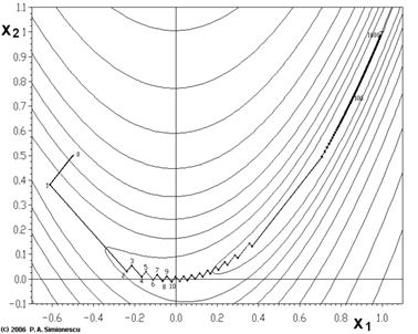
这幅图表示的是对一个目标函数的寻优过程，图中锯齿状的路线就是寻优路线在二维平面上的投影。
这个函数的表达式是：
f(x1,x2)=(1−x1)2+100⋅(x2−x12)2 
它叫做Rosenbrock function（罗森布罗克方程），是个非凸函数，在最优化领域，它通常被用来作为一个最优化算法的performance test函数。
我们来看一看它在三维空间中的图形：

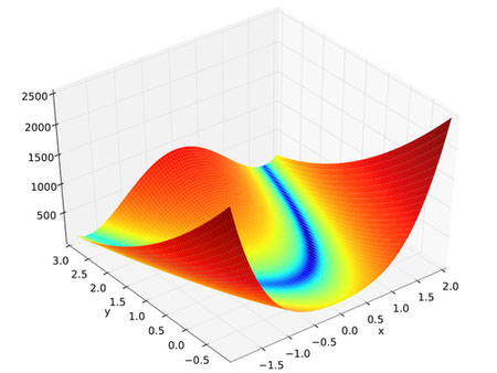
它的全局最优点位于一个长长的、狭窄的、抛物线形状的、扁平的“山谷”中。

找到“山谷”并不难，难的是收敛到全局最优解（全局最优解在 (1,1) 处）。

正所谓：世界上最遥远的距离，不是你离我千山万水，而是你就在我眼前，我却要跨越千万步，才能找到你。

我们再来看另一个目标函数 f(x,y)=sin(12x2−14y2+3)cos(2x+1−ey) 的寻优过程：

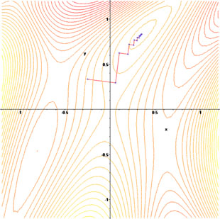
和前面的Rosenbrock function一样，它的寻优过程也是“锯齿状”的。
它在三维空间中的图形是这样的：

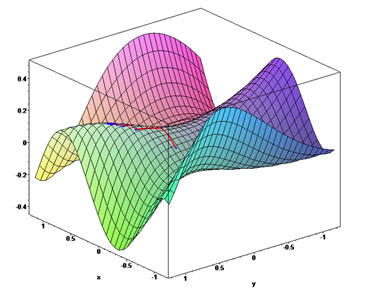
总而言之就是：当目标函数的等值线接近于圆(球)时，下降较快；等值线类似于扁长的椭球时，一开始快，后来很慢。

『5』为什么“慢”的分析
上面花花绿绿的图确实很好看，我们看到了那些寻优过程有多么“惨烈”——太艰辛了不是么？
但不能光看热闹，还要分析一下——为什么会这样呢？
由精确line search满足的一阶必要条件，得：
∇f(xk+αkdk)Tdk=0 ，即 gTk+1dk=0 
故由最速下降法的 dk=−gk 得：
gTk+1dk=gTk+1(−gk)=−gTk+1gk=−dTk+1dk=0⇒ dTk+1dk=0 
即：相邻两次的搜索方向是相互直交的（投影到二维平面上，就是锯齿形状了）。

如果你非要问，为什么 dTk+1dk=0 就表明这两个向量是相互直交的？那么我就耐心地再解释一下：
由两向量夹角的公式：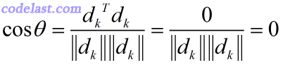

=> θ=π2 
两向量夹角为90度，因此它们直交。

 

『6』优点
这个被我们说得一无是处的最速下降法真的就那么糟糕吗？其实它还是有优点的：程序简单，计算量小；并且对初始点没有特别的要求；此外，许多算法的初始/再开始方向都是最速下降方向（即负梯度方向）。

『7』收敛性及收敛速度
最速下降法具有整体收敛性——对初始点没有特殊要求。
采用精确线搜索的最速下降法的收敛速度：线性。

采用 Levmar 工具包分析用代码：

#include "stdafx.h"
#include <stdio.h>
#include <stdlib.h>
#include <math.h>
#include <float.h>

#include "levmar.h"
#define ROSD 105.0

/* Rosenbrock function, global minimum at (1, 1) */
void ros(double *p, double *x, int m, int n, void *data)
{
    register int i;

    for (i = 0; i<n; ++i)
        x[i] = ((1.0 - p[0])*(1.0 - p[0]) + ROSD*(p[1] - p[0] * p[0])*(p[1] - p[0] * p[0]));
}

void jacros(double *p, double *jac, int m, int n, void *data)
{
    register int i, j;

    for (i = j = 0; i<n; ++i) {
        jac[j++] = (-2 + 2 * p[0] - 4 * ROSD*(p[1] - p[0] * p[0])*p[0]);
        jac[j++] = (2 * ROSD*(p[1] - p[0] * p[0]));
    }
}

#define MODROSLAM 1E02
/* Modified Rosenbrock problem, global minimum at (1, 1) */
void modros(double *p, double *x, int m, int n, void *data)
{
    register int i;

    for (i = 0; i<n; i += 3) {
        x[i] = 10 * (p[1] - p[0] * p[0]);
        x[i + 1] = 1.0 - p[0];
        x[i + 2] = MODROSLAM;
    }
}

void jacmodros(double *p, double *jac, int m, int n, void *data)
{
    register int i, j;

    for (i = j = 0; i<n; i += 3) {
        jac[j++] = -20.0*p[0];
        jac[j++] = 10.0;

        jac[j++] = -1.0;
        jac[j++] = 0.0;

        jac[j++] = 0.0;
        jac[j++] = 0.0;
    }
}

int main()
{
    register int i, j;
    int problem, ret;
    double p[5], // 5 is max(2, 3, 5)
        x[16]; // 16 is max(2, 3, 5, 6, 16)
    int m, n;
    double opts[LM_OPTS_SZ], info[LM_INFO_SZ];
    opts[0] = LM_INIT_MU; opts[1] = 1E-15; opts[2] = 1E-15; opts[3] = 1E-20;
    opts[4] = LM_DIFF_DELTA; // relevant only if the Jacobian is approximated using finite differences; specifies forward differencing 
                             //opts[4]=-LM_DIFF_DELTA; // specifies central differencing to approximate Jacobian; more accurate but more expensive to compute!

                             /* modified Rosenbrock problem */
    m = 2; n = 3;
    p[0] = -1.2; p[1] = 1.0;
    for (i = 0; i<n; i++) x[i] = 0.0;
    ret = dlevmar_der(modros, jacmodros, p, x, m, n, 1000, opts, info, NULL, NULL, NULL); // with analytic Jacobian
                                                                                          //ret=dlevmar_dif(modros, p, x, m, n, 1000, opts, info, NULL, NULL, NULL);  // no Jacobian
    printf("Levenberg-Marquardt returned %d in %g iter, reason %g\nSolution: ", ret, info[5], info[6]);
    for (i = 0; i<m; ++i)
        printf("%.7g ", p[i]);
    printf("\n\nMinimization info:\n");
    for (i = 0; i<LM_INFO_SZ; ++i)
        printf("%g ", info[i]);
    printf("\n");

    getchar();
    return 0;
}

运行结果：

可以可看到迭代了14次后，最终求出来的(x,y)已经非常接近（1,1）了。