吴恩达课程第二周01作业Python Basics with Numpy (optional assignment)

最新推荐文章于 2022-10-15 14:55:34 发布

编程的机械狗

最新推荐文章于 2022-10-15 14:55:34 发布

阅读量392

点赞数

分类专栏：吴恩达机器学习文章标签：机器学习 python

本文链接：https://blog.csdn.net/weixin_42326997/article/details/106753082

版权

吴恩达机器学习专栏收录该内容

3 篇文章 0 订阅

订阅专栏

Python Basics with Numpy (optional assignment)

1、sigmoid函数

也叫Logistic函数，用于隐层神经元输出，取值范围为(0,1)，它可以将一个实数映射到(0,1)的区间，可以用来做二分类。在特征相差比较复杂或是相差不是特别大时效果比较好。Sigmoid作为激活函数有以下优缺点：
优点：平滑、易于求导。
缺点：激活函数计算量大，反向传播求误差梯度时，求导涉及除法；反向传播时，很容易就会出现梯度消失的情况，从而无法完成深层网络的训练。
在这里插入图片描述

import numpy as np
import matplotlib.pyplot as plt
def sigmoid(x):
    return 1.0/(np.exp(-x)+1)
sigmoid_inputs = np.arange(-10,10,0.1)
sigmoid_outputs = sigmoid(sigmoid_inputs)
print("sigmoid Function 输入：：{}".format(sigmoid_inputs))
print("sigmoid Function 输出：：{}".format(sigmoid_outputs))
plt.plot(sigmoid_inputs,sigmoid_outputs)
plt.xlabel("sigmoid Inputs")
plt.ylabel("sigmoid Outputs")
plt.show()

在这里插入图片描述
可以看出，把（-10，10）之间的数都映射为（0，1）之间的数

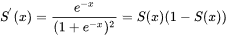
def sigmoid_derivative(x):
    s = sigmoid(x)
    ds = s*(1-s)
    return ds
sigmoid_gradient = sigmoid_derivative(sigmoid_inputs)
plt.plot(sigmoid_inputs,sigmoid_gradient)
plt.xlabel("sigmoid Inputs")
plt.ylabel("sigmoid Gradient")
plt.show()

在这里插入图片描述

2、归一化

我们在机器学习和深度学习中使用的另一个常见技术是规范化我们的数据。由于归一化后梯度下降收敛速度更快，因此通常会获得更好的性能。把x的每一行向量除以它的范数

2.1范数

范数是具有 “长度” 概念的函数，在数学上，范数包括向量范数和矩阵范数。向量范数表征向量空间中向量的大小，矩阵范数表征矩阵引起变化的大小。
一种非严密的解释就是，对应向量范数，向量空间中的向量都是有大小的，这个大小如何度量，就是用范数来度量的，不同的范数都可以来度量这个大小，就好比米和尺都可以来度量远近一样；对于矩阵范数，学过线性代数，我们知道，通过运算 AX=B，可以将向量 X 变化为 B，矩阵范数就是来度量这个变化大小的。向量的范数可以简单形象的理解为向量的长度，或者向量到零点的距离，或者相应的两个点之间的距离。
$l_{p}$ 范数的定义
$||x||_{p}=(\sum_{i=1}^n x_{i}^p)^\frac{1}{p}$

||x||、 ||X||，其中下x、X为向量和矩阵。表示向量x,矩阵X 的范数例如向量 $x=[1,-2,3]^T$ 的欧式范数 (Euclideannorm) 为 :
$||x||_{2}=\sqrt{1^2+(-2)^2+3^2}=3.742$

用于表示向量的大小，这个范数也被叫做 $l_{2}$ 范数。

常用的范数：

$l_{0}$ -范数：,表示的是向量x中非零元素的个数

$l_{1}$ -范数：,表示向量中所有元素绝对值之和。

$l_{2}$ -范数：表示向量（或矩阵）的元素平方和

2.2、使用np求范数

x_norm=np.linalg.norm(x, ord=None, axis=None, keepdims=False)

x: 表示矩阵（也可以是一维）

ord：范数类型
在这里插入图片描述

矩阵的范数：

ord=1：列和的最大值

ord=2： $λE-A^TA|=0$ ，求特征值，然后求最大特征值得算术平方根

ord=∞：行和的最大值

axis：处理类型

axis=1表示按行向量处理，求多个行向量的范数

axis=0表示按列向量处理，求多个列向量的范数

axis=None表示矩阵范数。

keepding：是否保持矩阵的二维特性

True表示保持矩阵的二维特性，False相反

x = np.array([[0,3,4],
             [1,6,4]])
print("默认参数：{}".format(np.linalg.norm(x)))
print("矩阵二范数，保留矩阵{}".format(np.linalg.norm(x,keepdims = True)))
print("矩阵的每个行向量求2范数{}".format(np.linalg.norm(x,axis =1,keepdims = True)))
print("矩阵的每个列向量求2范数{}".format(np.linalg.norm(x,axis =0,keepdims = True)))
print("*********************")
print("矩阵1范数{}".format(np.linalg.norm(x,ord = 1,keepdims = True)))
print("矩阵2范数{}".format(np.linalg.norm(x,ord = 2,keepdims = True)))
print("***********************")
print("矩阵每个行向量1范数{}".format(np.linalg.norm(x,ord = 1,axis=1,keepdims = True)))
print("矩阵每个列向量1范数{}".format(np.linalg.norm(x,ord = 1,axis=0,keepdims = True)))

在这里插入图片描述

2.3 矩阵的归一化

def normalizeRows(x):
    x_norm = np.linalg.norm(x,ord = 2,axis =1 ,keepdims = True)
    x = x/ x_norm
    return x
x = np.array([
    [0, 3, 4],
    [1, 6, 4]])
print(x)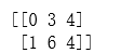

在这里插入图片描述

3． np.shape 于 np.reshape

在深度学习中使用的两个常见numpy函数是np.shape()以及np.reshape(). np.shape用于获取矩阵/向量X的形状（维度）。np.reshape()用于将X重塑为其他维度。
采用np.array()创建时需要几个维度就要用几个[ ]括起来，这种创建方式要给定数据；采用np.ones()或np.zeros()创建分别产生全1或全0的数据，用a.shape会输出你创建时的输入，创建时输入了几个维度输出就会用几个[ ]括起来，shape的返回值是一个元组，里面每个数字表示每一维的长度
np.shape[]是对应到某一维上输出指定维的长度
例如建立多维矩阵用np.ones()其中后两个参数代表先建立3行4列的二维矩阵，第二个参数代表有2个这样的二位数组，第一个参数代表有3个这样的三维数组。

a = np.ones([3,2,3,4])
print(a)

在这里插入图片描述

4、softmax

在机器学习尤其是深度学习中，softmax是个非常常用而且比较重要的函数，尤其在多分类的场景中使用广泛。他把一些输入映射为0-1之间的实数，并且归一化保证和为1，因此多分类的概率之和也刚好为1。

在这里插入图片描述

def softmax(x):
    x_exp = np.exp(x)
    x_exp_sum = np.sum(x_exp,axis = 1,keepdims = True)
    s =x/x_exp_sum
    return s
x = np.array([
    [9, 2, 5, 0, 0],
    [7, 5, 0, 0 ,0]])
print("softmax(x) = " + str(softmax(x)))

在这里插入图片描述

5、向量化

向量化是非常基础的去除代码中 for循环的艺术，在深度学习安全领域、深度学习实践中，你会经常发现自己训练大数据集，因为深度学习算法处理大数据集效果很棒，所以代码运行速度非常重要，否则如果在大数据集上，代码可能花费很长时间去运行，将要等待非常长的时间去得到结果。所以在深度学习领域，运行向量化是一个关键的技巧。
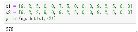
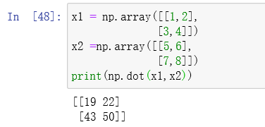
Np.dot()返回的是两个数组的点积(dot product)（对于矩阵和数组用法一样）
1.如果处理的是一维数组，则得到的是两数组的內积
在这里插入图片描述
2 如果是二维数组（矩阵）之间的运算，则得到的是矩阵积

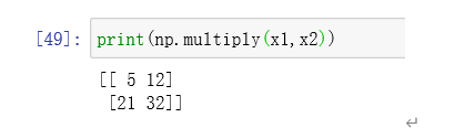
np.multiply()函数
函数作用数组和矩阵对应位置相乘，输出与相乘数组/矩阵的大小一致

*
对于数组是对应元素相成，矩阵来说执行矩阵乘法

总结一下：
dot对于矩阵和数组来说是一样的（矩阵乘法）

Multiply 对于矩阵和数组一样（对应元素相乘）

*对于矩阵来说是矩阵乘法，数组是逐个元素相乘。
在numpy中，array（实际上是ndarray，表示多维数组）是可以有多维度的，而matrix只有两个维度，即行和列。所以matrix是array的一种特例，因而它继承了array的所有函数，同时还特别为matrix开发了自己新的函数。简言之，array可以使用的函数，matrix都可以使用，而matrix可以使用的函数array未必可以使用。

作业的具体代码

print("Hello World")
print ("test:Hello world ")

# GRADED FUNCTION: basic_sigmoid
import math
def basic_sigmoid(x):
    """
    Compute sigmoid of x.
    Arguments:
    x -- A scalar
    Return:
    s -- sigmoid(x)
    """
    ### START CODE HERE ### (≈ 1 line of code)
    s =1/(1+math.exp(-x))
    ### END CODE HERE ###
    return s

basic_sigmoid(3)

### One reason why we use "numpy" instead of "math" in Deep Learning ###
x = [1, 2, 3]
basic_sigmoid(x) # you will see this give an error when you run it, because x is a vector.

import numpy as np
# example of np.exp
x = np.array([1, 2, 3])
print(np.exp(x)) # result is (exp(1), exp(2), exp(3))

# example of vector operation
x = np.array([1, 2, 3])
print (x + 3)

# GRADED FUNCTION: sigmoid
import numpy as np # this means you can access numpy functions by writing np.function() instead of numpy.function()
def sigmoid(x):
    """
    Compute the sigmoid of x
    Arguments:
    x -- A scalar or numpy array of any size
    Return:
    s -- sigmoid(x)
    """
    ### START CODE HERE ### (≈ 1 line of code)
    s = 1/(1+np.exp (-x))
    ### END CODE HERE ###
    return s

x = np.array([1, 2, 3])
sigmoid(x)

# GRADED FUNCTION: sigmoid_derivative
def sigmoid_derivative(x):
    """
    Compute the gradient (also called the slope or derivative) of the sigmoid function with respect to its input x.
    You can store the output of the sigmoid function into variables and then use it to calculate the gradient.
    Arguments:
    x -- A scalar or numpy array
    Return:
    ds -- Your computed gradient.
    """
    ### START CODE HERE ### (≈ 2 lines of code)
    s = sigmoid(x)
    ds = s*(1-s)
    ### END CODE HERE ###
    return ds

x = np.array([1, 2, 3])
print ("sigmoid_derivative(x) = " + str(sigmoid_derivative(x)))

# GRADED FUNCTION: image2vector
def image2vector(image):
    """
    Argument:
    image -- a numpy array of shape (length, height, depth)
    
    Returns:
    v -- a vector of shape (length*height*depth, 1)
    """
    
    ### START CODE HERE ### (≈ 1 line of code)
    v=image.reshape(image.shape[0]*image.shape[1]*image.shape[2],1)
    ### END CODE HERE ###
    
    return v

# This is a 3 by 3 by 2 array, typically images will be (num_px_x, num_px_y,3) where 3 represents the RGB values
image = np.array([[[ 0.67826139,  0.29380381],
        [ 0.90714982,  0.52835647],
        [ 0.4215251 ,  0.45017551]],
       [[ 0.92814219,  0.96677647],
        [ 0.85304703,  0.52351845],
        [ 0.19981397,  0.27417313]],
       [[ 0.60659855,  0.00533165],
        [ 0.10820313,  0.49978937],
        [ 0.34144279,  0.94630077]]])
print ("image2vector(image) = " + str(image2vector(image)))

# GRADED FUNCTION: normalizeRows
def normalizeRows(x):
    """
    Implement a function that normalizes each row of the matrix x (to have unit length).
    Argument:
    x -- A numpy matrix of shape (n, m)
    Returns:
    x -- The normalized (by row) numpy matrix. You are allowed to modify x.
    """
    ### START CODE HERE ### (≈ 2 lines of code)
    # Compute x_norm as the norm 2 of x. Use np.linalg.norm(..., ord = 2, axis = ..., keepdims = True)
    x_norm = np.linalg.norm(x,ord = 2,axis =1 ,keepdims = True)
    # Divide x by its norm.
    x = x/x_norm
    ### END CODE HERE ###
    return x

x = np.array([
    [0, 3, 4],
    [1, 6, 4]])
print("normalizeRows(x) = " + str(normalizeRows(x)))

# GRADED FUNCTION: softmax
def softmax(x):
    """Calculates the softmax for each row of the input x.
    Your code should work for a row vector and also for matrices of shape (n, m).
    Argument:
    x -- A numpy matrix of shape (n,m)v
    Returns:
    s -- A numpy matrix equal to the softmax of x, of shape (n,m)
    """ 
    ### START CODE HERE ### (≈ 3 lines of code)
    # Apply exp() element-wise to x. Use np.exp(...).
    x_exp = np.exp(x) 
    # Create a vector x_sum that sums each row of x_exp. Use np.sum(..., axis = 1, keepdims = True).
    x_sum = np.sum(x_exp,axis=1,keepdims=True)
    # Compute softmax(x) by dividing x_exp by x_sum. It should automatically use numpy broadcasting.
    s=x_exp/x_sum
    ### END CODE HERE ### 
    return s

# GRADED FUNCTION: L1
def L1(yhat, y):
    """
    Arguments:
    yhat -- vector of size m (predicted labels)
    y -- vector of size m (true labels)
    Returns:
    loss -- the value of the L1 loss function defined above
    """
    ### START CODE HERE ### (≈ 1 line of code)
    loss = np.sum(np.abs(y-yhat))
    ### END CODE HERE ###
    return loss

yhat = np.array([.9, 0.2, 0.1, .4, .9])
y = np.array([1, 0, 0, 1, 1])
print("L1 = " + str(L1(yhat,y)))

# GRADED FUNCTION: L2
def L2(yhat, y):
    """
    Arguments:
    yhat -- vector of size m (predicted labels)
    y -- vector of size m (true labels) 
    Returns:
    loss -- the value of the L2 loss function defined above
    """
    ### START CODE HERE ### (≈ 1 line of code)
    loss = np.sum(np.power((y-yhat),2))
    ### END CODE HERE ###
    return loss

yhat = np.array([.9, 0.2, 0.1, .4, .9])
y = np.array([1, 0, 0, 1, 1])
print("L2 = " + str(L2(yhat,y)))

编程的机械狗

关注

0
点赞
踩
2

收藏

觉得还不错? 一键收藏
0
评论
吴恩达课程第二周01作业Python Basics with Numpy (optional assignment)

Python Basics with Numpy (optional assignment)1、sigmoid函数也叫Logistic函数，用于隐层神经元输出，取值范围为(0,1)，它可以将一个实数映射到(0,1)的区间，可以用来做二分类。在特征相差比较复杂或是相差不是特别大时效果比较好。Sigmoid作为激活函数有以下优缺点：优点：平滑、易于求导。缺点：激活函数计算量大，反向传播求误差梯度时，求导涉及除法；反向传播时，很容易就会出现梯度消失的情况，从而无法完成深层网络的训练。import n
复制链接

扫一扫