数据分析-15-Bitcoin Historical Data比特币价格预测（包含代码数据）

0. 代码数据下载

关注公众号：『AI学习星球』
回复：比特币价格预测 即可获取数据下载。
算法学习、4对1辅导、论文辅导或核心期刊可以通过公众号或CSDN滴滴我

---

1. 导入包和数据

import numpy as np
import pandas as pd
import seaborn as sns
import matplotlib.pyplot as plt
import matplotlib as mpl
from scipy import stats
import statsmodels.api as sm
import warnings
from itertools import product
from datetime import datetime
warnings.filterwarnings('ignore')
plt.style.use('seaborn-poster')

df = pd.read_csv('bitstampUSD_1-min_data_2012-01-01_to_2021-03-31 2.csv')
df.head()

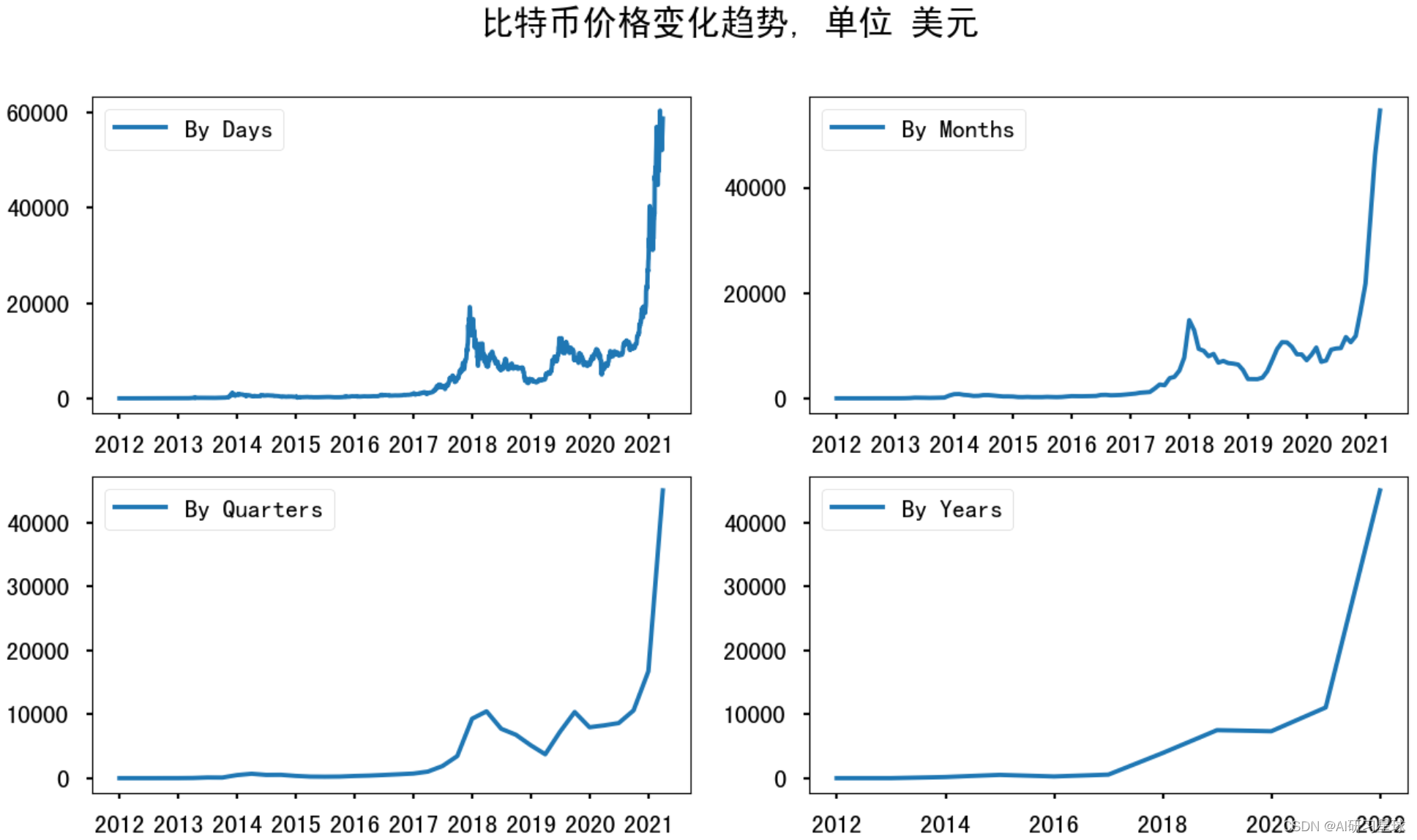
2.货币价格变化趋势分析

通过对数据库中四种因素来分别分析其对货币价格变化的影响并绘图

# 时间戳转化为日常时间格式
df.Timestamp = pd.to_datetime(df.Timestamp, unit='s')

# 对样本在不同时间频率上进行采样
df.index = df.Timestamp
df = df.resample('D').mean()

df_month = df.resample('M').mean()

df_year = df.resample('A-DEC').mean()

df_Q = df.resample('Q-DEC').mean()

# 中文乱码处理
plt.rcParams['font.sans-serif'] = ['SimHei']
plt.rcParams['axes.unicode_minus'] = False

# 绘图
fig = plt.figure(figsize=[15, 8])
plt.suptitle("比特币价格变化趋势, 单位 美元", fontsize=22)

plt.subplot(221)
plt.plot(df.Weighted_Price, '-', label='By Days')
plt.legend()

plt.subplot(222)
plt.plot(df_month.Weighted_Price, '-', label='By Months')
plt.legend()

plt.subplot(223)
plt.plot(df_Q.Weighted_Price, '-', label='By Quarters')
plt.legend()

plt.subplot(224)
plt.plot(df_year.Weighted_Price, '-', label='By Years')
plt.legend()

plt.show()

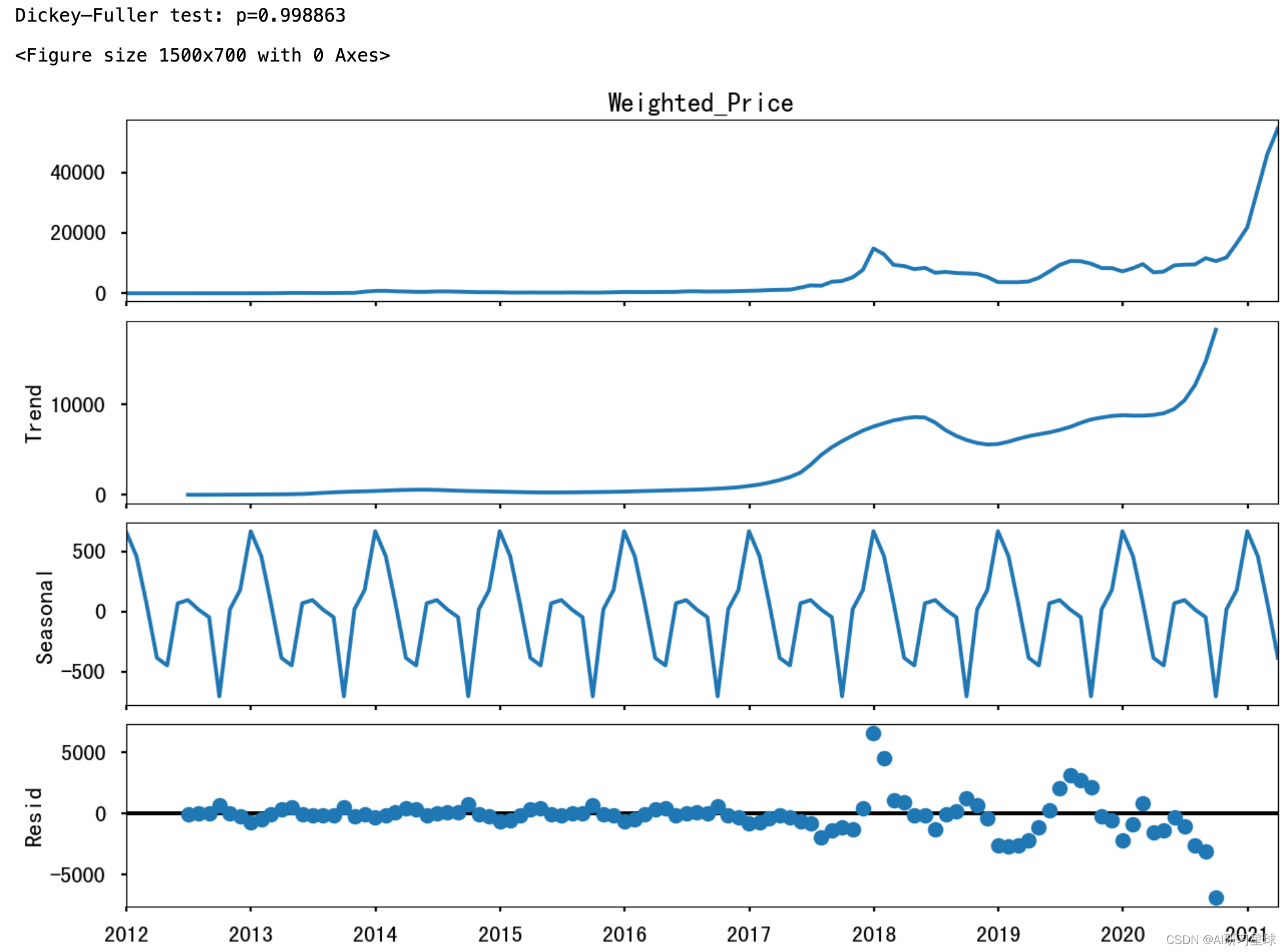
3. 稳定性检测与时间序列检测

对上述四种影响货币价格走向的四种因素分别进行稳定性与时间序列检测

plt.figure (figsize=[15, 7])
sm.tsa.seasonal_decompose(df_month.Weighted_Price).plot()
print("Dickey–Fuller test: p=%f" % sm.tsa.stattools.adfuller(df_month.Weighted_Price)[1])
plt.show()

4. 数据变化

由于连续的响应变量不满足正态分布，所以数据需要进行Box-Cox变换

df_month['Weighted_Price_box'], lmbda = stats.boxcox(df_month.Weighted_Price)
print("Dickey–Fuller test: p=%f" % sm.tsa.stattools.adfuller(df_month.Weighted_Price)[1])

Dickey–Fuller test: p=0.998863

由于时间序列季节对数据的影响，所以季节差异化需要考虑，代码如下：

df_month['prices_box_diff'] = df_month.Weighted_Price_box - df_month.Weighted_Price_box.shift(12)
print("Dickey–Fuller test: p=%f" % sm.tsa.stattools.adfuller(df_month.prices_box_diff[12:])[1])

Dickey–Fuller test: p=0.444282

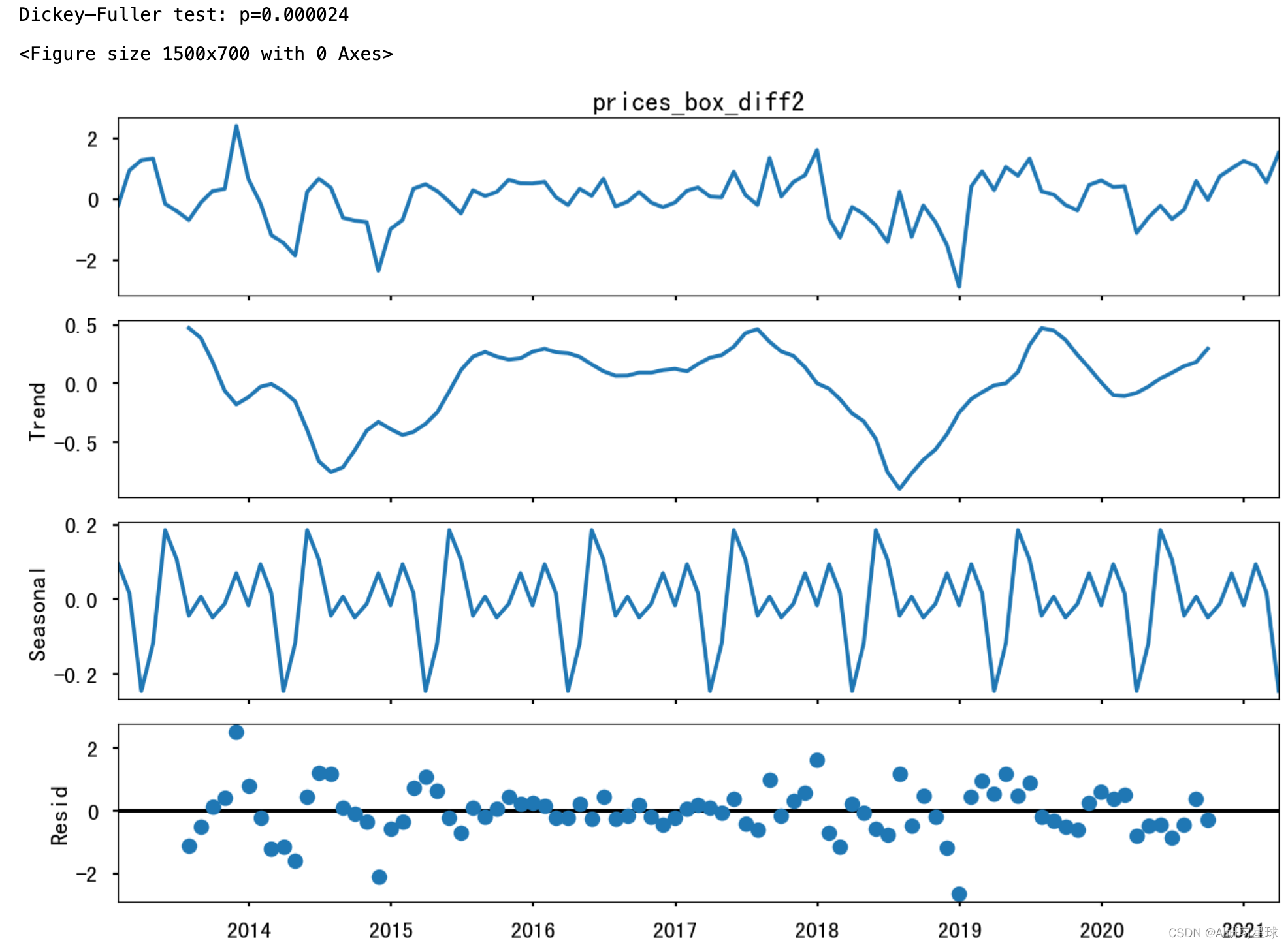
为减少数据的随机性与波动性，需要进行数据规律化分布，代码如下：

# Regular differentiation
df_month['prices_box_diff2'] = df_month.prices_box_diff - df_month.prices_box_diff.shift(1)
plt.figure(figsize=(15,7))

# STL-decomposition
sm.tsa.seasonal_decompose(df_month.prices_box_diff2[13:]).plot()   
print("Dickey–Fuller test: p=%f" % sm.tsa.stattools.adfuller(df_month.prices_box_diff2[13:])[1])

plt.show()

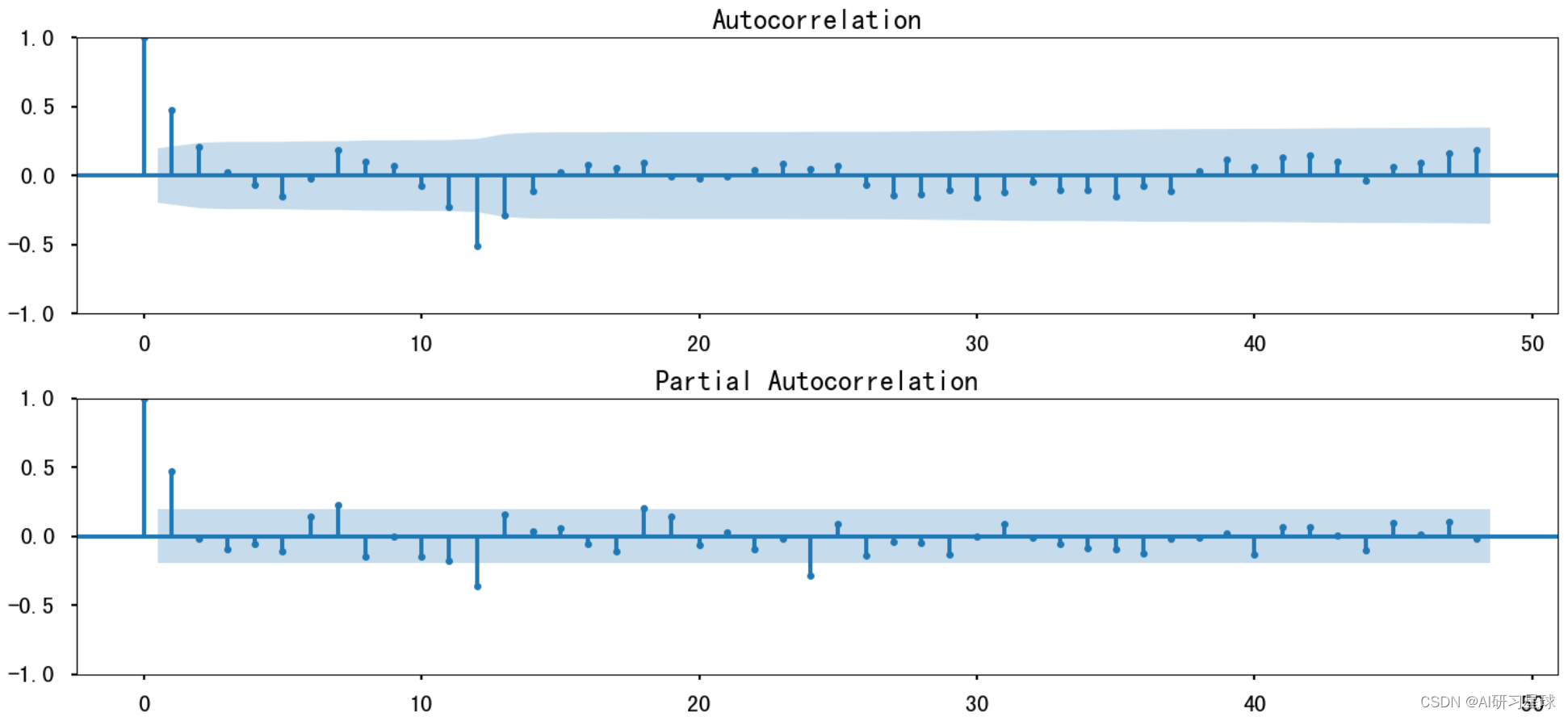
5. 模型分析

将处理完的数据导入对应的模型中，使用自相关和部分自相关图对参数进行初始近似处理

plt.figure(figsize=(15,7))
ax = plt.subplot(211)
sm.graphics.tsa.plot_acf(df_month.prices_box_diff2[13:].values.squeeze(), lags=48, ax=ax)
ax = plt.subplot(212)
sm.graphics.tsa.plot_pacf(df_month.prices_box_diff2[13:].values.squeeze(), lags=48, ax=ax)
plt.tight_layout()
plt.show()

参数初始化与模型选择代码如下：

# Initial approximation of parameters
Qs = range(0, 2)
qs = range(0, 3)
Ps = range(0, 3)
ps = range(0, 3)
D=1
d=1
parameters = product(ps, qs, Ps, Qs)
parameters_list = list(parameters)
len(parameters_list)

# Model Selection
results = []
best_aic = float("inf")
warnings.filterwarnings('ignore')
for param in parameters_list:
    try:
        model=sm.tsa.statespace.SARIMAX(df_month.Weighted_Price_box, order=(param[0], d, param[1]), 
                                        seasonal_order=(param[2], D, param[3], 12)).fit(disp=-1)
    except ValueError:
        print('wrong parameters:', param)
        continue
    aic = model.aic
    if aic < best_aic:
        best_model = model
        best_aic = aic
        best_param = param
    results.append([param, model.aic])

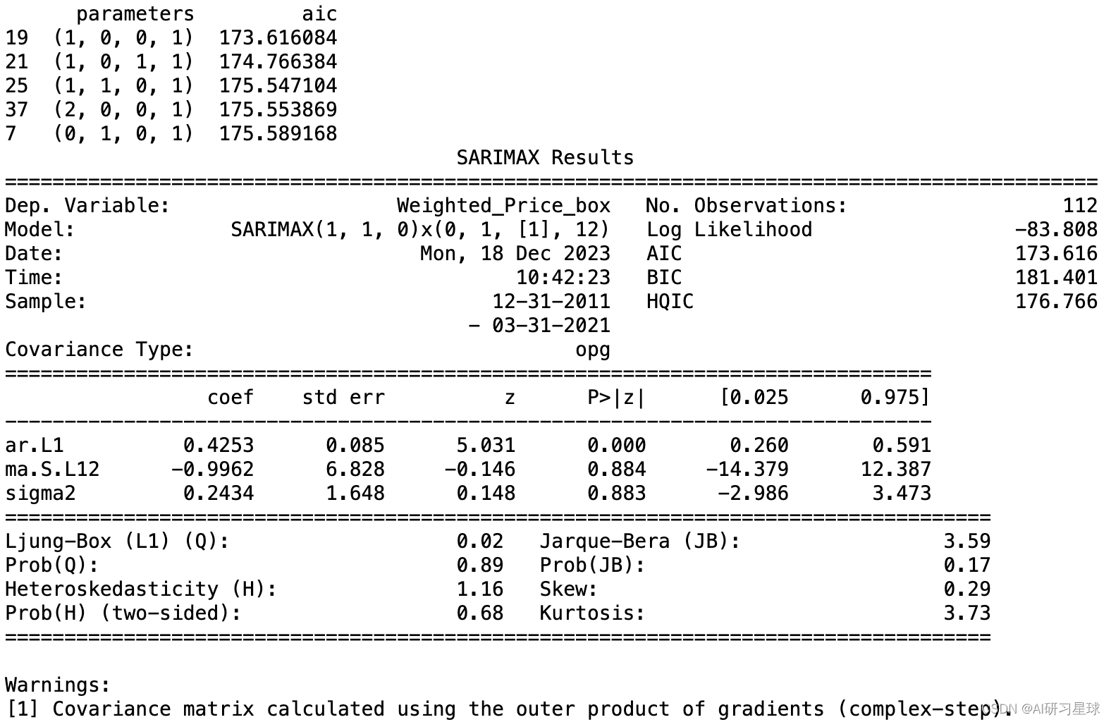
result_table = pd.DataFrame(results)
result_table.columns = ['parameters', 'aic']
print(result_table.sort_values(by = 'aic', ascending=True).head())
print(best_model.summary())

参数与建模结果如所示：

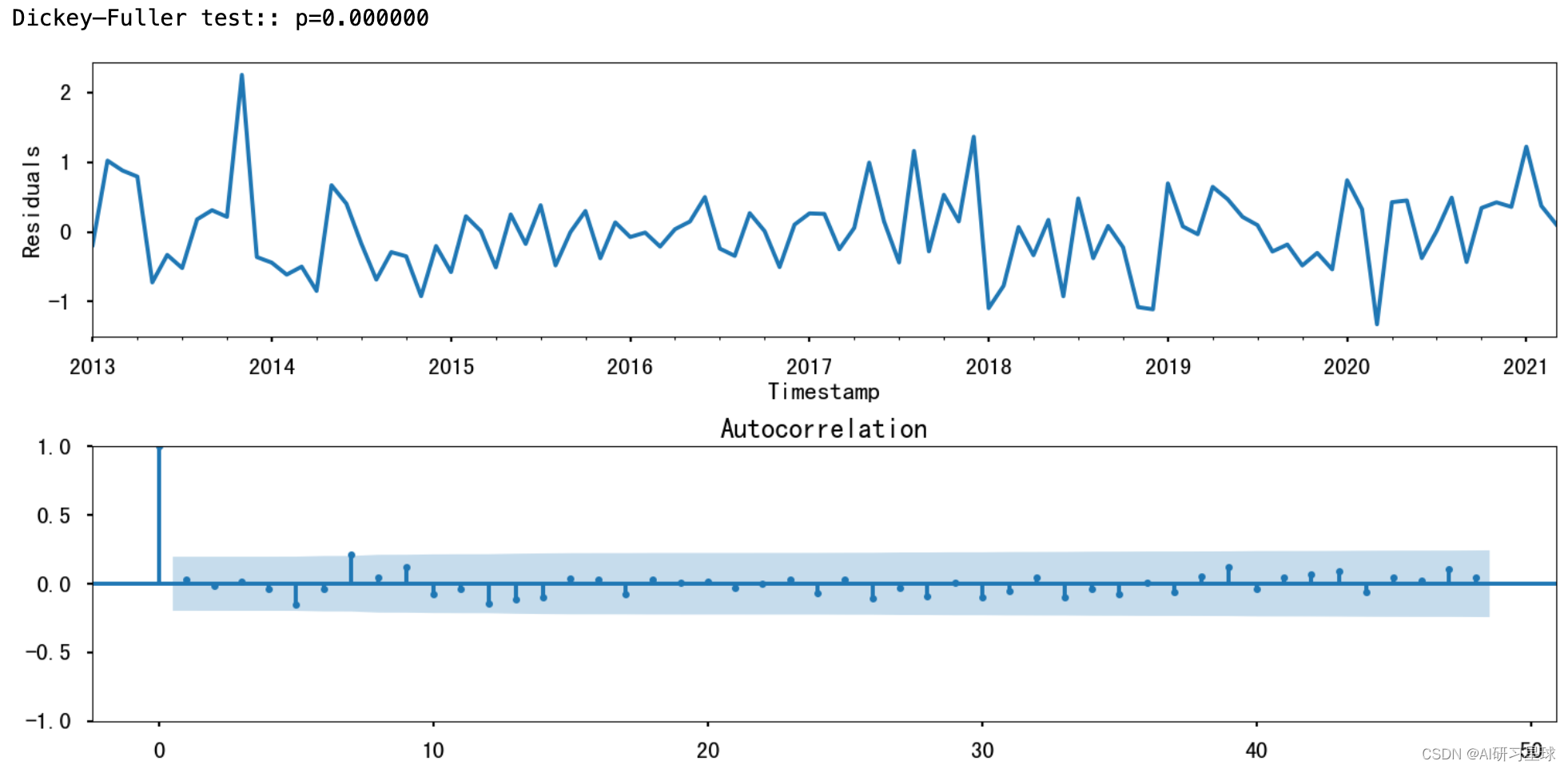
6. 残留物分析

使用STL分解法对残留物进行分析

# STL-decomposition
plt.figure(figsize=(15,7))
plt.subplot(211)
best_model.resid[13:].plot()
plt.ylabel(u'Residuals')
ax = plt.subplot(212)
sm.graphics.tsa.plot_acf(best_model.resid[13:].values.squeeze(), lags=48, ax=ax)

print("Dickey–Fuller test:: p=%f" % sm.tsa.stattools.adfuller(best_model.resid[13:])[1])

plt.tight_layout()
plt.show()

7. 预测

根据前六步得到的分析数据与模型结果，基于时间序列与四种因素对比特币价格进行预测，并与实际价格趋势曲线进行拟合对比

def invboxcox(y,lmbda):
   if lmbda == 0:
      return(np.exp(y))
   else:
      return(np.exp(np.log(lmbda*y+1)/lmbda))

# 预测
df_month2 = df_month[['Weighted_Price']]
date_list = [datetime(2017, 6, 30), datetime(2017, 7, 31), datetime(2017, 8, 31), datetime(2017, 9, 30), 
             datetime(2017, 10, 31), datetime(2017, 11, 30), datetime(2017, 12, 31), datetime(2018, 1, 31),
             datetime(2018, 1, 28)]
future = pd.DataFrame(index=date_list, columns= df_month.columns)
df_month2 = pd.concat([df_month2, future])
df_month2['forecast'] = invboxcox(best_model.predict(start=0, end=75), lmbda)
plt.figure(figsize=(15,7))
df_month2.Weighted_Price.plot()
df_month2.forecast.plot(color='r', ls='--', label='Predicted Weighted_Price')
plt.legend()
plt.rcParams['font.sans-serif'] =['SimHei']
plt.rcParams['axes.unicode_minus'] = False
plt.title('比特币涨势, 月份')
plt.ylabel('mean USD')
plt.show()

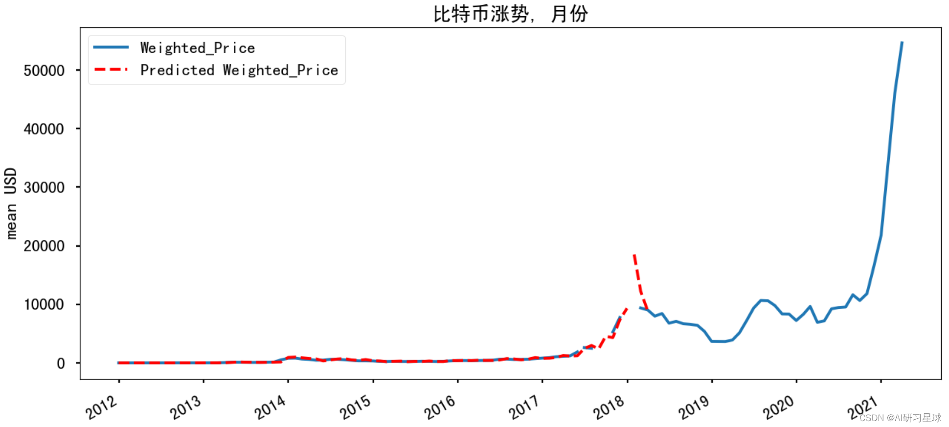
分析：由图可见，实际曲线与预测曲线拟合较好，说明模型的优越性，预测算法的准确性，有着较好的预测效果。

---

关注公众号：『AI学习星球』
回复：比特币价格预测 即可获取数据下载。
算法学习、4对1辅导、论文辅导或核心期刊可以通过公众号或CSDN滴滴我