python实现表格线性回归_python简单实现线性回归案例（linear_regression）

这个案例先自己造了一个线性回归的轮子，然后对比python自带库进行对比，代码放出来，亲测可行：

# %load ../../standard_import.txt

import pandas as pd

import numpy as np

import matplotlib.pyplot as plt

from sklearn.linear_model import LinearRegression

from mpl_toolkits.mplot3d import axes3d

pd.set_option('display.notebook_repr_html', False)

pd.set_option('display.max_columns', None)

pd.set_option('display.max_rows', 150)

pd.set_option('display.max_seq_items', None)

# %config InlineBackend.figure_formats = {'pdf',}

import seaborn as sns

sns.set_context('notebook')

sns.set_style('white')

def warmUpExercise():

return(np.identity(5))

warmUpExercise()

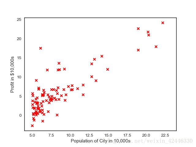
data = np.loadtxt('linear_regression_data1.txt', delimiter=',')

X = np.c_[np.ones(data.shape[0]),data[:,0]]

y = np.c_[data[:,1]]

plt.scatter(X[:,1], y, s=30, c='r', marker='x', linewidths=1)

plt.xlim(4,24)

plt.xlabel('Population of City in 10,000s')

plt.ylabel('Profit in $10,000s');

plt.show()

# 计算损失函数

def computeCost(X, y, theta=[[0], [0]]):

m = y.size

J = 0

h = X.dot(theta)

J = 1.0 / (2 * m) * (np.sum(np.square(h - y)))

return J

s = computeCost(X,y)

print s

# 梯度下降

def gradientDescent(X, y, theta=[[0], [0]], alpha=0.01, num_iters=1500):

m = y.size

J_history = np.zeros(num_iters)

for iter in np.arange(num_iters):

h = X.dot(theta)

theta = theta - alpha * (1.0 / m) * (X.T.dot(h - y))

J_history[iter] = computeCost(X, y, theta)

return (theta, J_history)

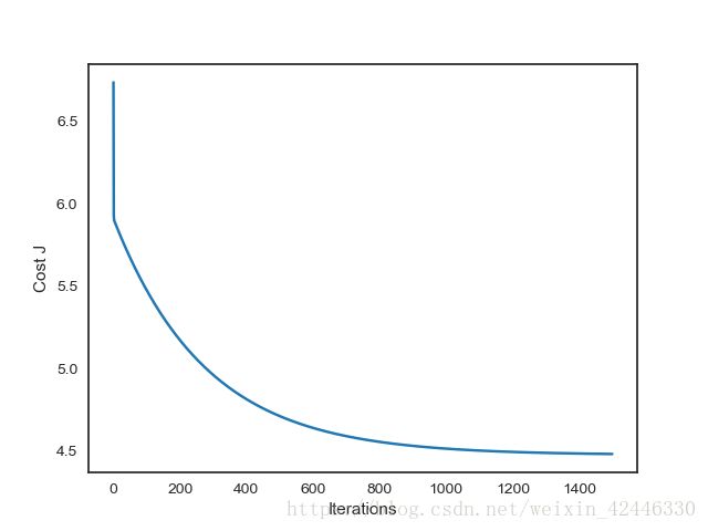
# 画出每一次迭代和损失函数变化

theta , Cost_J = gradientDescent(X, y)

print('theta: ',theta.ravel())

plt.plot(Cost_J)

plt.ylabel('Cost J')

plt.xlabel('Iterations');

plt.show()

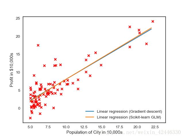
xx = np.arange(5,23)

yy = theta[0]+theta[1]*xx

# 画出我们自己写的线性回归梯度下降收敛的情况

plt.scatter(X[:,1], y, s=30, c='r', marker='x', linewidths=1)

plt.plot(xx,yy, label='Linear regression (Gradient descent)')

# 和Scikit-learn中的线性回归对比一下

regr = LinearRegression()

regr.fit(X[:,1].reshape(-1,1), y.ravel())

plt.plot(xx, regr.intercept_+regr.coef_*xx, label='Linear regression (Scikit-learn GLM)')

plt.xlim(4,24)

plt.xlabel('Population of City in 10,000s')

plt.ylabel('Profit in $10,000s')

plt.legend(loc=4);

plt.show()

# 预测一下人口为35000和70000的城市的结果

print(theta.T.dot([1, 3.5])*10000)

print(theta.T.dot([1, 7])*10000)

最终输出结果如下：

运行结果：

32.072733877455676

('theta: ', array([-3.63029144,  1.16636235]))

[4519.7678677]

[45342.45012945]