一些常用的python绘图包

置顶星尘逸风

已于 2022-05-05 10:14:51 修改

阅读量3.4k

点赞数 1

分类专栏：算法 base 文章标签： python 数据分析

于 2022-02-09 22:40:49 首次发布

本文链接：https://blog.csdn.net/weixin_42394432/article/details/122851271

版权

算法同时被 2 个专栏收录

17 篇文章 2 订阅

订阅专栏

base

7 篇文章 0 订阅

订阅专栏

最后更新
2022.02.12

绘图库大全：
matplotlib底层灵活可实现复杂操作
seaborn是mp的上层更简单
pyecharts百度的图表可视化库
basemap地理地图
pygal矢量图
networkx网络
plotly地图趋势
turtle作画
mayavi三维可视化
opengl开放图形库
其他的还有pyqtgraph、pyQT5、PIL（pillow）、tkinter、holoviews、altair、vispy、bokeh等

matplotlib

一般用import matplotlib.pyplot as plt；import numpy as np
而pylab是把上两个都包含了，快速开发简单的可以用，复杂的还是不用pylab，调用耗时
matplotlib.patches包是形状，但不常用

点线

在这里插入图片描述

import matplotlib.pyplot as plt
import numpy as np

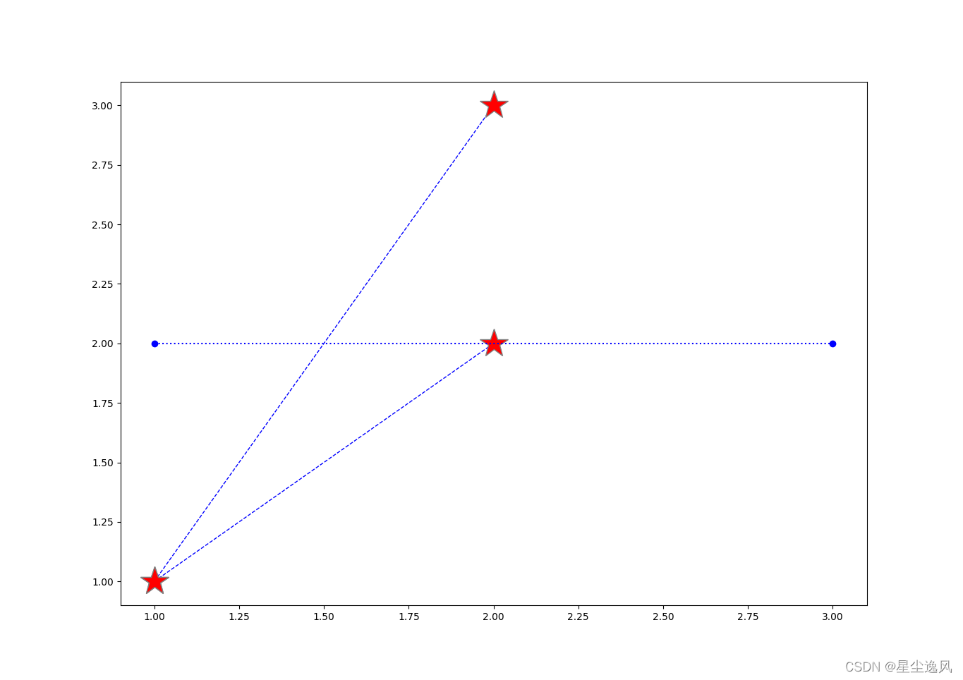
plt.plot( [1,2],[1,2],'--b',[1,2],[1,3], '--b', label='curve_fit values', linewidth=1) # 可以同时传多个xy组
plt.plot( [1,2],[1,2], '*r',[1,2],[1,3], '*r', label='original values',markersize=30
          , markeredgewidth=1, markeredgecolor="grey")  # 可以不传x，默认012递增
# markeredgewidth点边缘的大小和颜色
plt.plot([1,3],[2,2],'ob:')  # o原点 :点线
# 第三个参数传参 点型marker= 颜色color= 线型linestyle=
# 点 常用的，><v^ 方向三角、s方块、1234 方向Y、p五边形、hH六边形、o圆形、D棱形、 . - | + x *
# 色 c青cyan、r红red、g绿green、b蓝blue、w白white、k黑black、y黄yellow、m洋红magenta  或 #FF0000 red也可以
# 线 :点线、-.点画线、--虚线、-实线
plt.show()

在这里插入图片描述

import matplotlib.pyplot as plt
import numpy as np

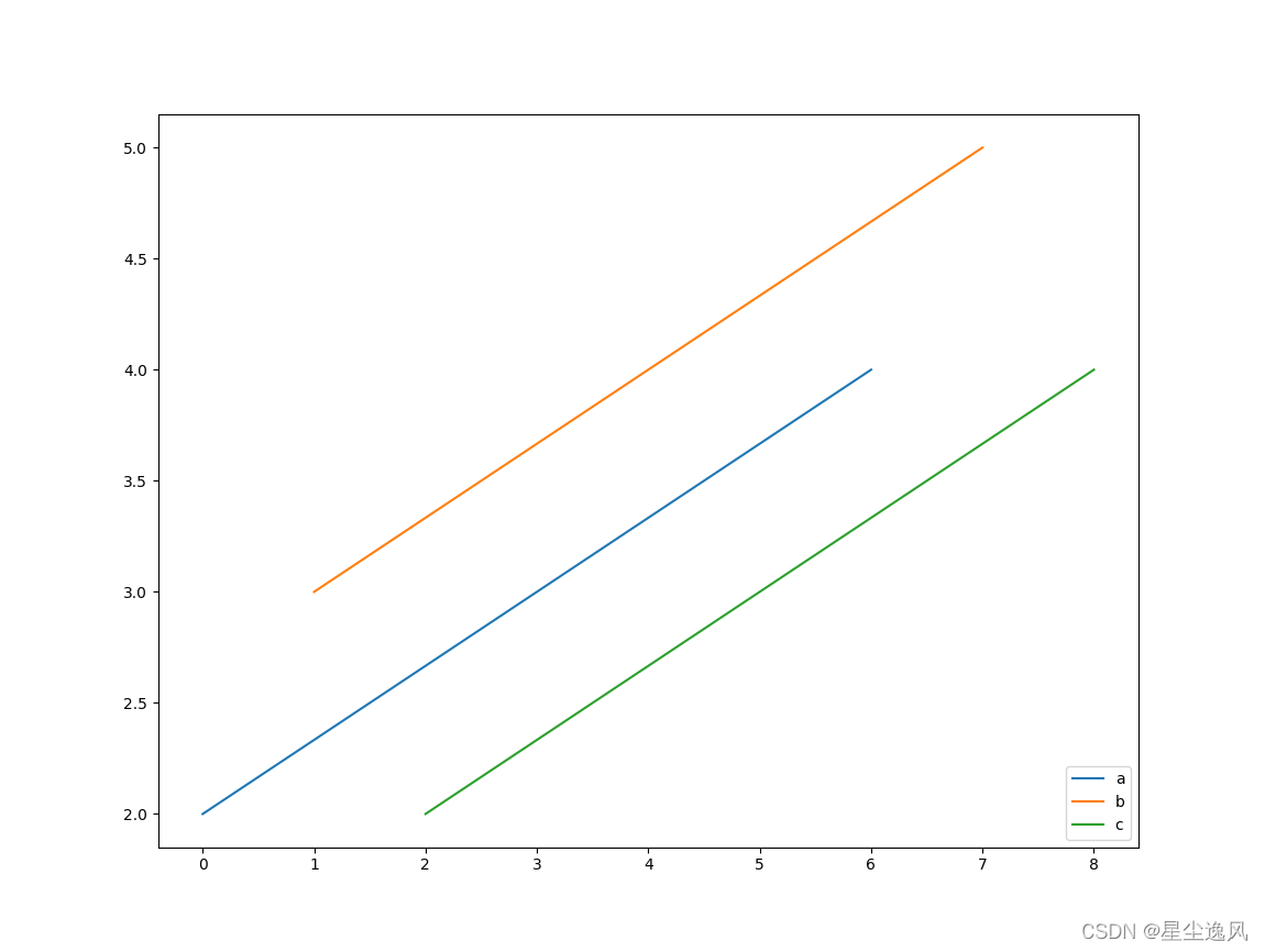
x=np.array([[0,1,2],[3,4,5],[6,7,8]])
y=np.array([[2,3,2],[3,4,3],[4,5,4]])
plt.plot(x,y)  # 传多维数组自动给不同的颜色
plt.legend(['a','b','c'],loc=4)  # 按顺序分配label，loc标记说明是在第几象限角
plt.show()

散点

在这里插入图片描述

import matplotlib.pyplot as plt
import numpy as np


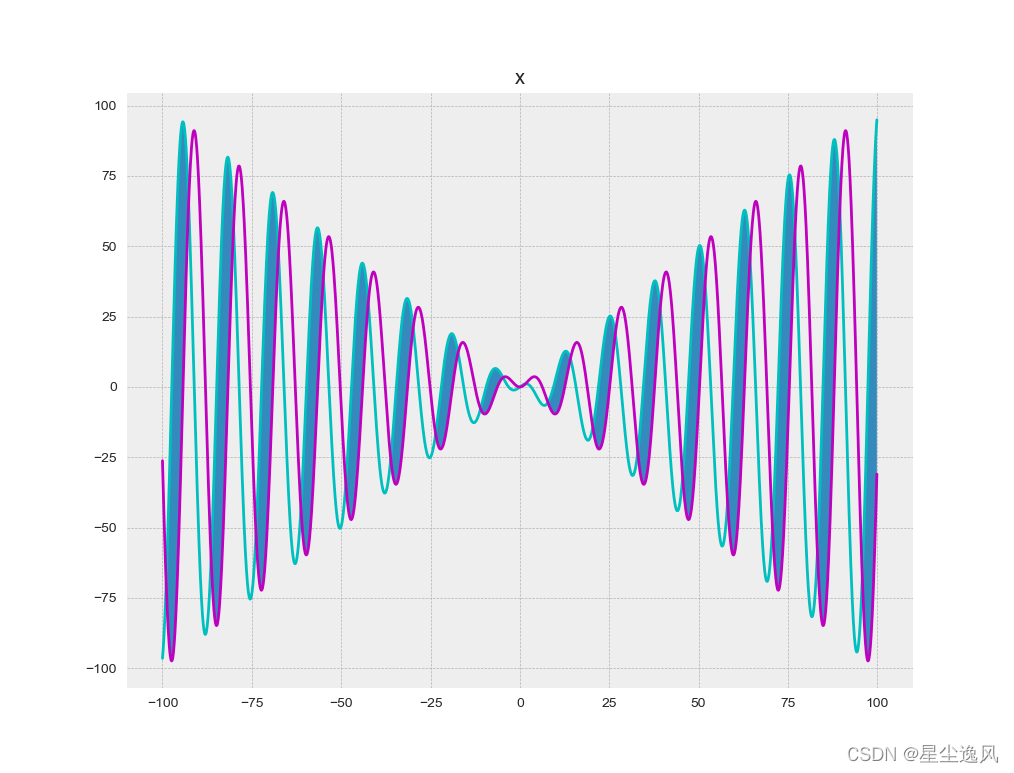
x=np.arange(-100,100,0.1)
plt.title('x')
plt.plot(x,x*np.cos(x),'c')
plt.plot(x,x*np.sin(x),'g')
plt.show()
exit()
# 3 散点
n = 10 # 用于生成十个点
x = np.random.rand(n)
y = np.random.rand(n)
# x=[2,3,4,5,26,2,11,22]
# y=[2,23,24,5,5,33,6,20]
plt.scatter(x,y,200,'r','*',alpha=0.6,linewidths=1,edgecolors='g')   # x,y,点大小，颜色，样式，透明度0-1,边缘大小，颜色
plt.show()
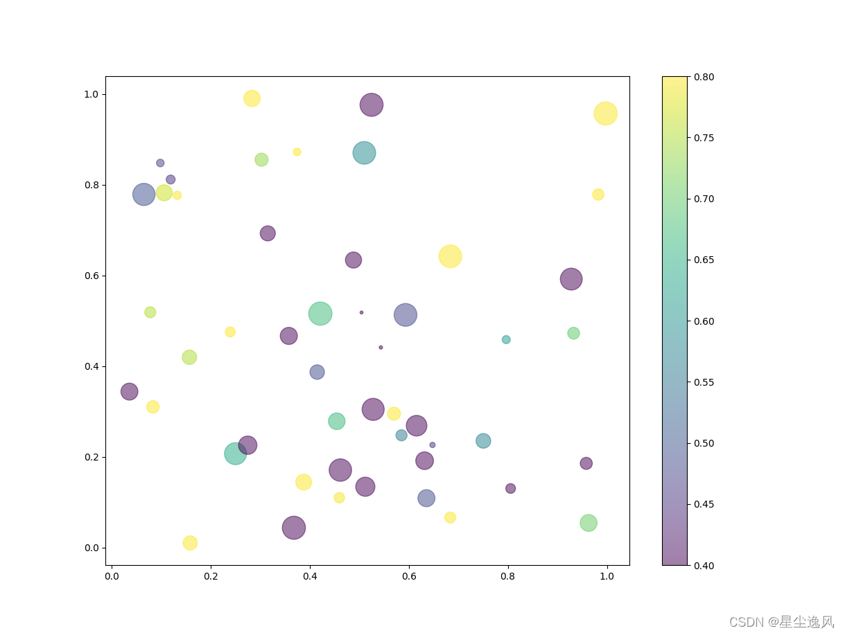
n = 50
x = np.random.rand(n)
y = np.random.rand(n)
q = np.random.rand(n)
w = np.random.rand(n)
from matplotlib import colors  # 调整色盘
changecolor = colors.Normalize(vmin=0.4, vmax=0.8)
plt.scatter(x,y,q*600,w,'o',alpha=0.5, cmap='viridis',norm=changecolor)
# 颜色映射cmap可能的取值：
# Accent, Accent_r, Blues, Blues_r, BrBG, BrBG_r, BuGn, BuGn_r, BuPu, BuPu_r, CMRmap, CMRmap_r, Dark2, Dark2_r,
# GnBu, GnBu_r, Greens, Greens_r, Greys, Greys_r, OrRd, OrRd_r, Oranges, Oranges_r, PRGn, PRGn_r, Paired, Paired_r,
# Pastel1, Pastel1_r, Pastel2, Pastel2_r, PiYG, PiYG_r, PuBu, PuBuGn, PuBuGn_r, PuBu_r, PuOr, PuOr_r, PuRd, PuRd_r,
# Purples, Purples_r, RdBu, RdBu_r, RdGy, RdGy_r, RdPu, RdPu_r, RdYlBu, RdYlBu_r, RdYlGn, RdYlGn_r, Reds, Reds_r,
# Set1, Set1_r, Set2, Set2_r, Set3, Set3_r, Spectral, Spectral_r, Wistia, Wistia_r, YlGn, YlGnBu, YlGnBu_r, YlGn_r,
# YlOrBr, YlOrBr_r, YlOrRd, YlOrRd_r, afmhot, afmhot_r, autumn, autumn_r, binary, binary_r, bone, bone_r, brg,
# brg_r, bwr, bwr_r, cividis, cividis_r, cool, cool_r, coolwarm, coolwarm_r, copper, copper_r, cubehelix, cubehelix_r,
# flag, flag_r, gist_earth, gist_earth_r, gist_gray, gist_gray_r, gist_heat, gist_heat_r, gist_ncar, gist_ncar_r,
# gist_rainbow, gist_rainbow_r, gist_stern, gist_stern_r, gist_yarg, gist_yarg_r, gnuplot, gnuplot2, gnuplot2_r,
# gnuplot_r, gray, gray_r, hot, hot_r, hsv, hsv_r, inferno, inferno_r, jet, jet_r, magma, magma_r, nipy_spectral,
# nipy_spectral_r, ocean, ocean_r, pink, pink_r, plasma, plasma_r, prism, prism_r, rainbow, rainbow_r, seismic,
# seismic_r, spring, spring_r, summer, summer_r, tab10, tab10_r, tab20, tab20_r, tab20b, tab20b_r, tab20c, tab20c_r,
# terrain, terrain_r, viridis, viridis_r, winter, winter_r
plt.colorbar()  # 显示颜色条
plt.show()

样式

在这里插入图片描述

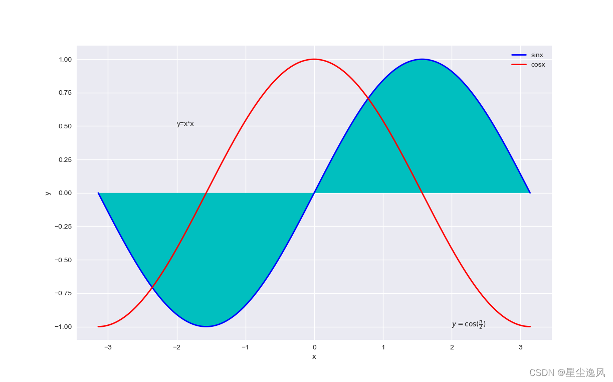
plt.style.use('seaborn') # 设置样式，bmh也好看，plt.style.available查看所有样式
plt.figure(figsize=(10,5)) # 创建绘图对象，figsize尺寸
subplot(1,1,1)  # 子图只有一块
x = np.linspace(-np.pi, np.pi, 256, endpoint=True) # 创建等差一维数组
y1 = np.sin(x)
y2 = np.cos(x)
plt.plot(x,y1,color='b',linewidth=2.0,linestyle="-",label = "sinx")
plt.plot(x,y2,color='r',linewidth=2.0,linestyle="-",label = "cosx")
plt.text(-2,0.5,'y=x*x')
plt.text(2,-1,r'$ y=\cos(\frac{\pi}{2}) $')  # 数学公式
# plt.grid(axis='x',linestyle='--')  # 显示网格，可以不传参
plt.xlabel('x')
plt.ylabel('y')
# plt.locator_params(nbins=20)  #  调整坐标轴刻度数量
# plt.xlim(xmin=10,xmax=25) # 坐标轴范围
plt.fill(x,y1,'c')  # 填充
plt.legend(loc='best')  # 自动选最好的位置
plt.show()

在这里插入图片描述

# 填充
plt.style.use('bmh')
x=np.arange(-100,100,0.1)
y1=x*np.cos(x/5)
y2=x*np.sin(x/5)
plt.plot(x,y1,'c')
plt.plot(x,y2,'g')
plt.fill_between(x,y1,y2) # 填充函数交叉区域
plt.show()

坐标系

在这里插入图片描述

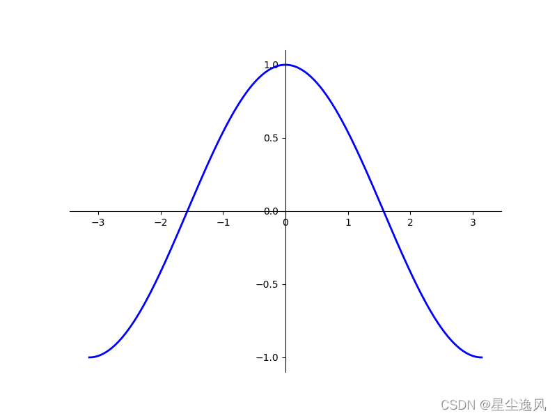
from pylab import *
figure(figsize=(8,6))
x = linspace(-np.pi, np.pi, 250,endpoint=True)
plot(x, cos(x), color="b", linewidth=2, linestyle="-")
ax = gca()  # 设置坐标系
ax.spines['right'].set_color('none')
ax.spines['top'].set_color('none')
ax.spines['bottom'].set_position(('data',0))  # 调整到0位置
ax.spines['left'].set_position(('data',0))
yticks([-1,-0.5, 0,0.5, 1])  # 轴记号
show()

数学之心

在这里插入图片描述

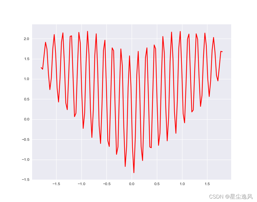
from pylab import *
style.use('seaborn')
x = linspace(-2, 2, 140,endpoint=True)
z=abs(x)**(2/3)+0.8*sqrt(3.3-x**2)*sin(1100*pi*x)
plot(x, z, color="r", linewidth=2, linestyle="-")
show()

等高线

在这里插入图片描述

from pylab import *
n = 1000
# 栅格化：两组1000个-3到3的一维数组成x和y，会形成1000*1000个焦点的二维数组
x, y = meshgrid(np.linspace(-3, 3, n),linspace(-3, 3, n))
print(x.shape,y.shape)  # (1000, 1000) (1000, 1000)
y1 = np.random.uniform(0.5, 1.0, n)    # 均匀分布随机数
y2 = np.random.uniform(0.5, 1.0, n)
z = (1 - x/2 + x**5 + y**3) * np.exp(-x**2 - y**2)
# 绘制图像
cntr = contour(x, y, z, 8, colors='black', linewidths=0.5)  # 线型，虚线是负的，实线是正的
# 创建标签
clabel(cntr, inline_spacing=1, fmt='%.1f', fontsize=10)  # 对象，线内宽，文字格式，文字大小
# 色带型等高线对象
cntr = contourf(x, y, z, 8, cmap='jet')  # 色带型
show()

热力图

在这里插入图片描述

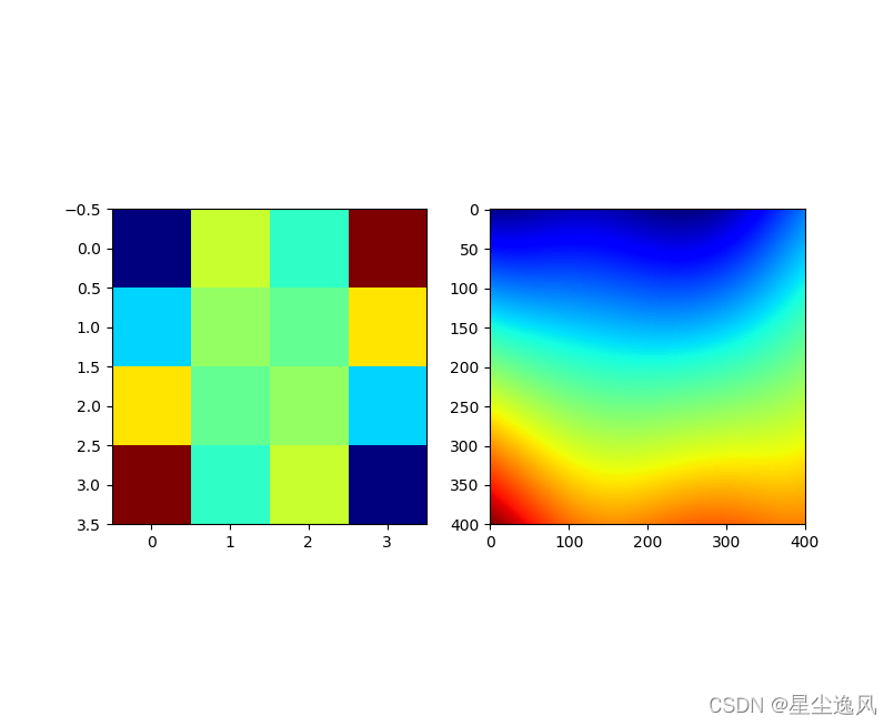
from pylab import *
subplot(121)
X,Y = np.meshgrid(np.linspace(-3,3,4),np.linspace(-3,3,4))
imshow(X*Y*cos(X), cmap='jet')
subplot(122)
x,y = np.meshgrid(np.linspace(-3,3,400),np.linspace(-3,3,400))
imshow(x*y*cos(x)+x**2+y/0.1, cmap='jet')
show()

饼图

在这里插入图片描述

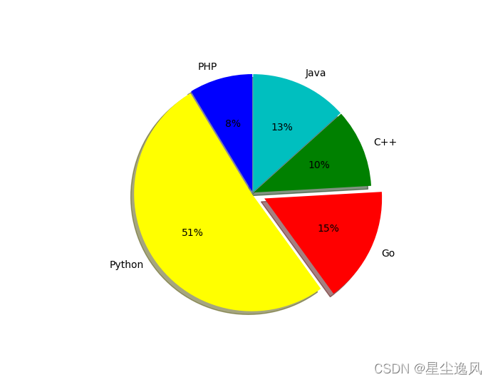
from pylab import *
# 值 间隙 标签 颜色列表,格式,shadow=阴影, startangle=起始角度
pie([17, 100, 31, 21, 26],
    [0.01, 0.01, 0.11, 0.01, 0.01],
    ['PHP', 'Python', 'Go', 'C++', 'Java'],
    ['blue', 'yellow', 'red', 'green','c'],
    '%d%%',shadow=True,startangle=90)
show()

分图显示

在这里插入图片描述

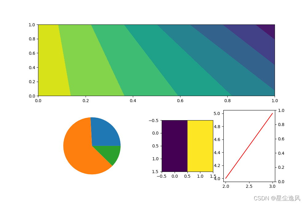
from pylab import *
subplot(2,1,1)  # 分2的1
contourf(array([[33,11],[33,-3]]))
subplot(2,2,3)  # 分4的3
pie([23,55,11])
subplot(2,4,7)  # 分8的7
imshow([[3,4],[3,4]])
subplot(2,4,8)
plot([2,3],[4,5],'r')
twinx()  # 增加x坐标系
show()

scatter 3D

在这里插入图片描述

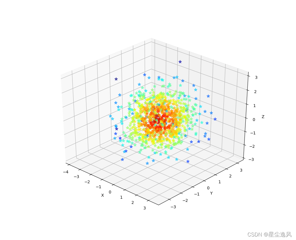
from pylab import *
from mpl_toolkits.mplot3d import axes3d
# 获得1000个使用随机作为服从正态分布的数据数组
n = 1000
x = np.random.normal(0, 1, n)
y = np.random.normal(0, 1, n)
z = np.random.normal(0, 1, n)
d = np.sqrt(x ** 2 + y ** 2 + z ** 2)
ax =gca(projection='3d')
ax.set_xlabel('X')
ax.set_ylabel('Y')
ax.set_zlabel('Z')
ax.scatter(x, y, z, s=60, c=d, cmap="jet_r", alpha=0.6, marker='*')
# axis('off')  # 去掉坐标
show()

wireframe 3D

在这里插入图片描述

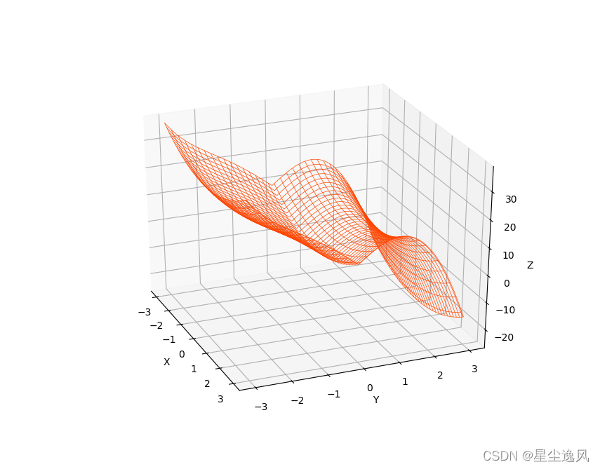
from pylab import *
from mpl_toolkits.mplot3d import axes3d
# 获得1000个使用随机作为服从正态分布的数据数组
n = 1000
x, y = np.meshgrid(np.linspace(-3, 3, n), np.linspace(-3, 3, n))
y1 =  np.random.uniform(0.5, 1.0, n)
y2 =  np.random.uniform(0.5, 1.0, n)
z =(x**2 - y**3+abs(sin(y))*10)
ax =gca(projection='3d')
ax.set_xlabel('X')
ax.set_ylabel('Y')
ax.set_zlabel('Z')
ax.plot_wireframe(x, y, z, rstride=30, cstride=30, linewidth=0.5, color='c')
# axis('off')  # 去掉坐标
show()

surface 3D

在这里插入图片描述

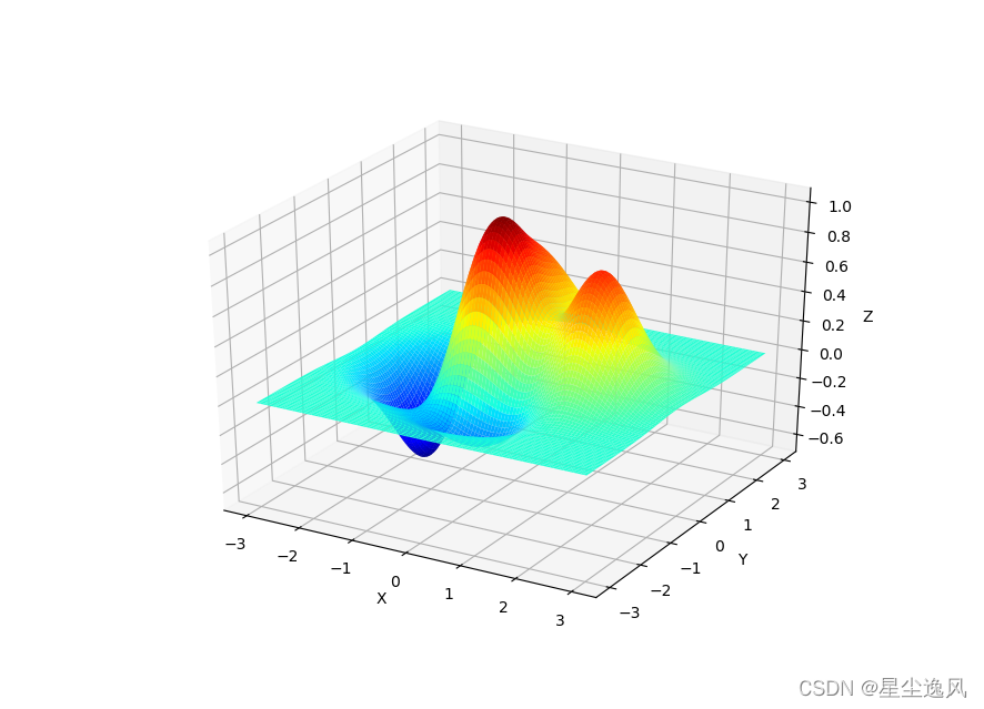
from pylab import *
from mpl_toolkits.mplot3d import axes3d
# 获得1000个使用随机作为服从正态分布的数据数组
n = 1000
x, y = np.meshgrid(np.linspace(-3, 3, n), np.linspace(-3, 3, n))
y1 =  np.random.uniform(0.5, 1.0, n)
y2 =  np.random.uniform(0.5, 1.0, n)
z = (1 - x/2 + x**5 + y**3) * np.exp(-x**2 - y**2)
ax =gca(projection='3d')
ax.set_xlabel('X')
ax.set_ylabel('Y')
ax.set_zlabel('Z')
ax.plot_surface(x, y, z, rstride=10, cstride=10, cmap='jet')
# axis('off')  # 去掉坐标
show()

contour 3D

在这里插入图片描述

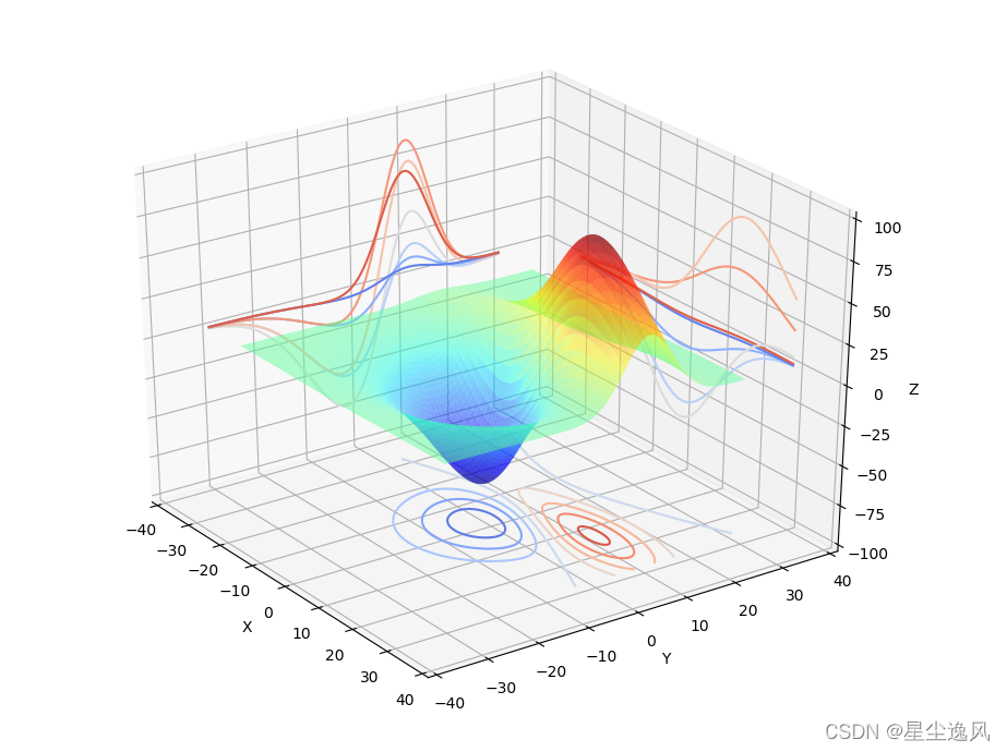
from mpl_toolkits.mplot3d import Axes3D
from matplotlib import cm
from mpl_toolkits.mplot3d import axes3d
fig = plt.figure()
ax = fig.gca(projection='3d')
X, Y, Z = axes3d.get_test_data(0.01)
ax.plot_surface(X, Y, Z, rstride=8, cstride=8, alpha=0.5, cmap='jet')
cset = ax.contour(X, Y, Z, zdir='z', offset=-100, cmap=cm.coolwarm)
cset = ax.contour(X, Y, Z, zdir='x', offset=-40, cmap=cm.coolwarm)
cset = ax.contour(X, Y, Z, zdir='y', offset=40, cmap=cm.coolwarm)
ax.set_xlabel('X')
ax.set_xlim(-40, 40)
ax.set_ylabel('Y')
ax.set_ylim(-40, 40)
ax.set_zlabel('Z')
ax.set_zlim(-100, 100)
plt.show()

经济柱形图

在这里插入图片描述

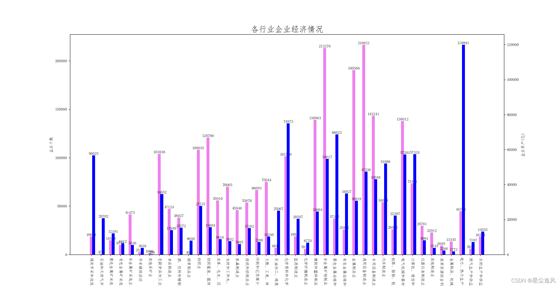
# 工业企业经济指标，数据来源-国家统计局-经济普查
b=pd.read_excel('jj.xls')
bb=np.array(b)
print(bb.shape)
print(bb[5:-3])  # (50-5-3, 7) 行业，企业数，资产，资本，主营，附加，从业人员

from pylab import *
# style.use('seaborn')
title('各行业企业经济情况',fontsize=20)
rcParams['font.sans-serif'] = ['FangSong']  # 指定默认字体,显示中文
lb=bb[6:-3][:,0]
lens=len(lb)
bar(range(0,lens*2,2),bb[6:-3][:,1],label=lb,color='violet',width=0.6,alpha=1)
# 添加数据标签在柱子上
for a, b in zip(range(0,lens*2,2),bb[6:-3][:,1]):
    plt.text(a, b + 0.05, '%.0f' % b, ha='center', va='bottom', fontsize=10)
xticks([i for i in range(0,lens*2,2)],lb,rotation=270)
ylabel('企业个数')

twinx()  # 增加坐标系
ylabel('企业资产(亿)')
bar([i+0.5 for i in range(0,lens*2,2)],bb[6:-3][:,2],color='b',width=0.6,alpha=1)
# 添加数据标签在柱子上
for a,c in zip(range(0,lens*2,2),bb[6:-3][:,2]):
    plt.text(a+0.5, c + 0.05, '%.0f' % c, ha='center', va='bottom', fontsize=10)

# legend()
show()

人口柱形图

在这里插入图片描述

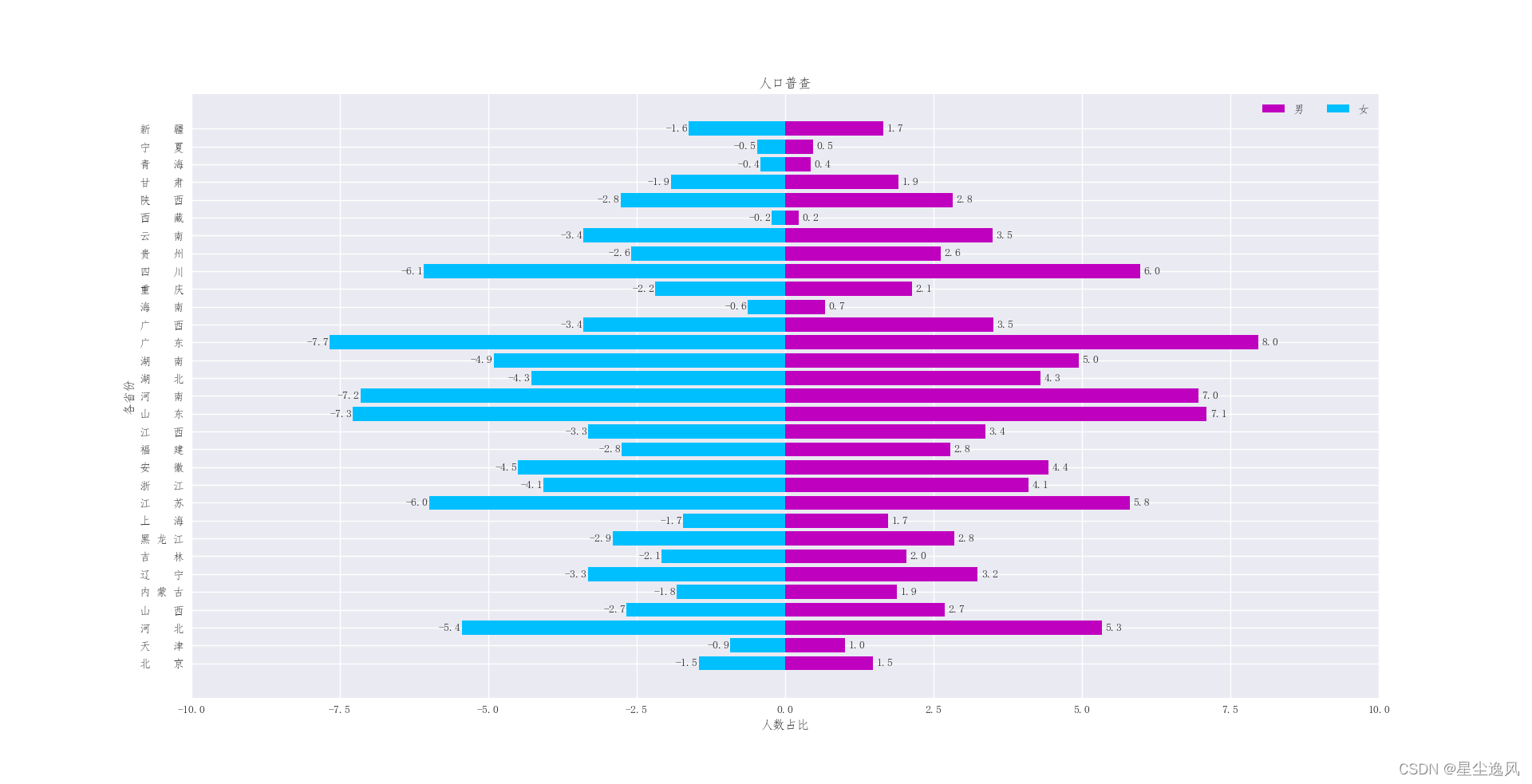
# 按地区的人口分布，数据来源-国家统计局-人口普查
a=pd.read_excel('man.xls')
print(a)
aa=np.array(a)
print(aa.shape)
print(aa[6:])  # (38-6, 17) 省，合计户数，家庭 集体 合计人数 男 女 性别比7  人/户-1
aasum=aa[6]
aa=aa[7:,:8]

from pylab import *
style.use('seaborn')
title('人口普查')
rcParams['font.sans-serif'] = ['FangSong']  # 指定默认字体,显示中文
rcParams['axes.unicode_minus'] = False  # 解决负数乱码
lb=aa[:,0]  # 省标签
lens=aa.shape[0]  # 数据条数
barh(lb,aa[:,5]/aasum[5]*100,label='男',color='m')  # 占总人数百分比
barh(lb,-aa[:,6]/aasum[6]*100,label='女',color='deepskyblue')
for a, b,c in zip(range(lens),-aa[:,6]/aasum[6]*100,aa[:,5]/aasum[5]*100):
    plt.text(b-0.2 ,a, round(b,1), ha='center', va='center', fontsize=10)
    plt.text(c+0.2 ,a, round(c,1), ha='center', va='center', fontsize=10)
xlim(-10,10)
xlabel('人数占比')
ylabel('各省份')
legend(loc="upper",ncol=2,frameon=False)
show()

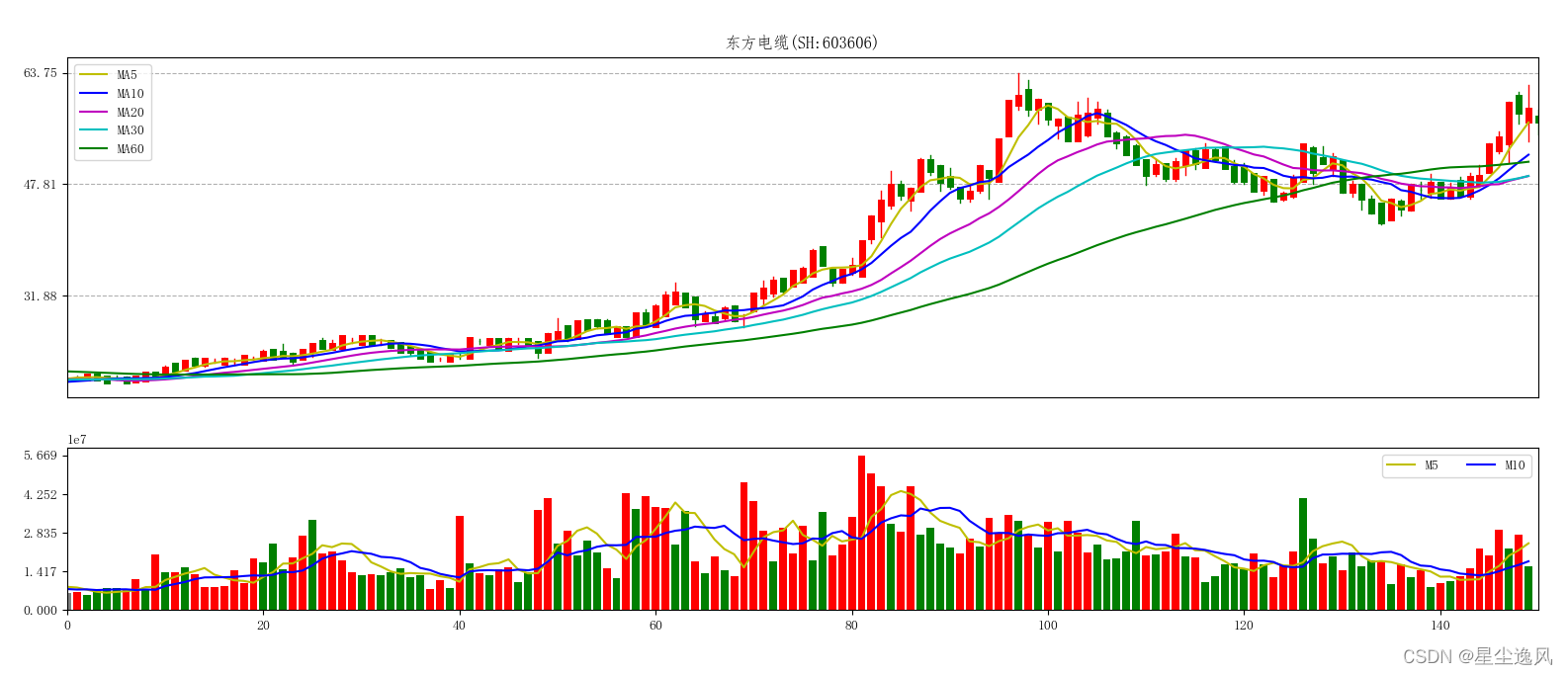
股票图

在这里插入图片描述

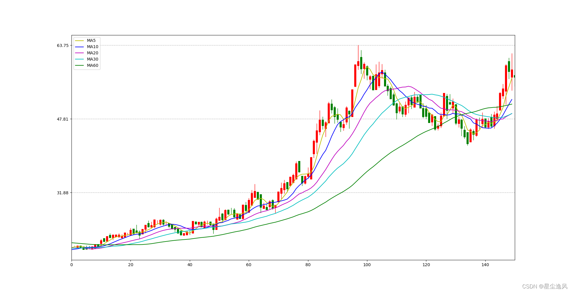
# 股票图，数据来源-同花顺软件
c=pd.read_csv('df.csv',encoding='gbk')
cc=np.array(c)
# print(cc)
print(cc.shape)  # (1774, 11) 日期 开盘 最高 最低 收盘4 涨幅 振幅 手7 金额 换手 成交
# 计算5 10 20 30 60日线  黄 蓝 粉 橙 绿
d5,d10,d20,d30,d60=[],[],[],[],[]
sp=cc[:,4]  # 收
rule = re.compile(r",")  # 8,023,778 <class 'str'>
hp=[int(rule.sub('', i)) for i in cc[:,7]]  # 手
M5,M10=[],[]
for i in range(150):
    d5.append(sum(sp[-150-5+i:-150+i])/5)
    d10.append(sum(sp[-150-10+i:-150+i])/10)
    d20.append(sum(sp[-150-20+i:-150+i])/20)
    d30.append(sum(sp[-150-30+i:-150+i])/30)
    d60.append(sum(sp[-150-60+i:-150+i])/60) 
    M5.append(sum(hp[-150-5+i:-150+i])/5)
    M10.append(sum(hp[-150-10+i:-150+i])/10)

cc=cc[-150:]
from pylab import *
rcParams['font.sans-serif'] = ['FangSong']  # 指定默认字体,显示中文
subplot(2,1,1)
title('东方电缆(SH:603606)')
n=0  # 对应取下标 日期
low,up=0,0
usec=[]
for i in cc:
    n+=1
    # print(i[1:5])
    k,g,d,s=i[1:5]
    if k<s:color='r'
    if k>s:color='green'
    if k==s:color='gray'
    usec.append(color)
    plot([n,n],[k,s],color,linewidth=5)
    plot([n,n],[min(k,s),d],color,linewidth=1)
    plot([n,n],[max(k,s),g],color,linewidth=1)
    low,up=min(low,d),max(up,g)
yticks(linspace(low,up,5,endpoint=True))  # 分为5等分价格
grid(linestyle='--',axis='y')
xlim(0,n)
# # 5 10 20 30 60日线  黄 蓝 粉 橙 绿
plot(range(150),d5,'-y',label='MA5')
plot(range(150),d10,'-b',label='MA10')
plot(range(150),d20,'-m',label='MA20')
plot(range(150),d30,'-c',label='MA30')
plot(range(150),d60,'-g',label='MA60')
legend()
xticks([])

subplot(4,1,3)
# 总手
hand=cc[:,7]
print(hand[4],type(hand[4]))
rule = re.compile(r",")  # 8,023,778 <class 'str'>
hand=[int(rule.sub('', i)) for i in hand]
hup=max( hand)
yticks(linspace(1,hup,5,endpoint=True))  # 分为5等分
for i in range(150):
    bar(i,int(hand[i]),color=usec[i])
xlim(0,n)
plot(range(150),M5,'-y',label='M5')
plot(range(150),M10,'-b',label='M10')
legend(ncol=2)

# subplot(4,1,3) # MACD未完待续
show()
exit()

在这里插入图片描述

turtle

它是是py自带包，海龟作图

bdd

图

import turtle

turtle.title('zzz') # 窗口名称
turtle.speed(5000)  # 画笔速度

# 左手外
turtle.penup() # 抬笔
turtle.goto(177, 112) # 到坐标
turtle.pencolor("lightgray")  # 亮灰色
turtle.pensize(3)  # 粗细
turtle.fillcolor("white")  # 填充色
turtle.begin_fill()  # 准备填充
turtle.pendown()  # 落笔
turtle.setheading(80)  # 转80度方向
turtle.circle(-45, 200) # 45半径右转200°
turtle.circle(-300, 23)
turtle.end_fill()  # 填充结束
# 左手内黑
turtle.penup()
turtle.goto(182, 95)
turtle.pencolor("black")
turtle.pensize(1)
turtle.fillcolor("black")
turtle.begin_fill()
turtle.setheading(95)
turtle.pendown()
turtle.circle(-37, 160)
turtle.circle(-20, 50)
turtle.circle(-200, 30)
turtle.end_fill()

# 下面全是用上面这些方法

# 身体外轮廓
# 从头顶左开始
turtle.penup()
turtle.goto(-73, 230)
turtle.pencolor("lightgray")
turtle.pensize(3)
turtle.fillcolor("white")
turtle.begin_fill()
turtle.pendown()
turtle.setheading(20)
turtle.circle(-250, 35)
# 左耳
turtle.setheading(50)
turtle.circle(-42, 180)
# 左侧
turtle.setheading(-50)
turtle.circle(-190, 30)
turtle.circle(-320, 45)
# 左腿
turtle.circle(120, 30)
turtle.circle(200, 12)
turtle.circle(-18, 85)
turtle.circle(-180, 23)
turtle.circle(-20, 110)
turtle.circle(15, 115)
turtle.circle(100, 12)
# 右腿
turtle.circle(15, 120)
turtle.circle(-15, 110)
turtle.circle(-150, 30)
turtle.circle(-15, 70)
turtle.circle(-150, 10)
turtle.circle(200, 35)
turtle.circle(-150, 20)
# 右手
turtle.setheading(-120)
turtle.circle(50, 30)
turtle.circle(-35, 200)
turtle.circle(-300, 23)
# 右侧
turtle.setheading(86)
turtle.circle(-300, 26)
# 右耳
turtle.setheading(122)
turtle.circle(-53, 160)
turtle.end_fill()


# 右耳内
turtle.penup()
turtle.goto(-137, 170)
turtle.pencolor("black")
turtle.pensize(1)
turtle.fillcolor("black")
turtle.begin_fill()
turtle.pendown()
turtle.setheading(120)
turtle.circle(-37, 160)
turtle.setheading(210)
turtle.circle(160, 20)
turtle.end_fill()

# 左耳内
turtle.penup()
turtle.goto(90, 230)
turtle.setheading(40)
turtle.begin_fill()
turtle.pendown()
turtle.circle(-30, 170)
turtle.setheading(125)
turtle.circle(150, 23)
turtle.end_fill()

# 右手内
turtle.penup()
turtle.goto(-180, -55)
turtle.fillcolor("black")
turtle.begin_fill()
turtle.setheading(-120)
turtle.pendown()
turtle.circle(50, 30)
turtle.circle(-27, 200)
turtle.circle(-300, 20)
turtle.setheading(-90)
turtle.circle(300, 14)
turtle.end_fill()

# 左腿内
turtle.penup()
turtle.goto(110, -173)
turtle.fillcolor("black")
turtle.begin_fill()
turtle.pendown()
turtle.setheading(-115)
turtle.circle(110, 15)
turtle.circle(200, 10)
turtle.circle(-18, 80)
turtle.circle(-180, 13)
turtle.circle(-20, 90)
turtle.circle(15, 60)
turtle.setheading(42)
turtle.circle(-200, 29)
turtle.end_fill()
# 右腿内
turtle.penup()
turtle.goto(-40, -215)
turtle.fillcolor("black")
turtle.begin_fill()
turtle.pendown()
turtle.setheading(-155)
turtle.circle(15, 100)
turtle.circle(-10, 110)
turtle.circle(-100, 30)
turtle.circle(-15, 65)
turtle.circle(-100, 10)
turtle.circle(200, 15)
turtle.setheading(-14)
turtle.circle(-200, 27)
turtle.end_fill()

# 右眼
# 眼圈
turtle.penup()
turtle.goto(-64, 120)
turtle.begin_fill()
turtle.pendown()
turtle.setheading(40)
turtle.circle(-35, 152)
turtle.circle(-100, 50)
turtle.circle(-35, 130)
turtle.circle(-100, 50)
turtle.end_fill()
# 眼珠
turtle.penup()
turtle.goto(-47, 55)
turtle.fillcolor("white")
turtle.begin_fill()
turtle.pendown()
turtle.setheading(0)
turtle.circle(25, 360)
turtle.end_fill()
turtle.penup()
turtle.goto(-45, 62)
turtle.pencolor("darkslategray")
turtle.fillcolor("darkslategray")
turtle.begin_fill()
turtle.pendown()
turtle.setheading(0)
turtle.circle(19, 360)
turtle.end_fill()
turtle.penup()
turtle.goto(-45, 68)
turtle.fillcolor("black")
turtle.begin_fill()
turtle.pendown()
turtle.setheading(0)
turtle.circle(10, 360)
turtle.end_fill()
turtle.penup()
turtle.goto(-47, 86)
turtle.pencolor("white")
turtle.fillcolor("white")
turtle.begin_fill()
turtle.pendown()
turtle.setheading(0)
turtle.circle(5, 360)
turtle.end_fill()

# 左眼
# 眼圈
turtle.penup()
turtle.goto(51, 82)
turtle.fillcolor("black")
turtle.begin_fill()
turtle.pendown()
turtle.setheading(120)
turtle.circle(-32, 152)
turtle.circle(-100, 55)
turtle.circle(-25, 120)
turtle.circle(-120, 45)
turtle.end_fill()
# 眼珠
turtle.penup()
turtle.goto(79, 60)
turtle.fillcolor("white")
turtle.begin_fill()
turtle.pendown()
turtle.setheading(0)
turtle.circle(24, 360)
turtle.end_fill()
turtle.penup()
turtle.goto(79, 64)
turtle.pencolor("darkslategray")
turtle.fillcolor("darkslategray")
turtle.begin_fill()
turtle.pendown()
turtle.setheading(0)
turtle.circle(19, 360)
turtle.end_fill()
turtle.penup()
turtle.goto(79, 70)
turtle.fillcolor("black")
turtle.begin_fill()
turtle.pendown()
turtle.setheading(0)
turtle.circle(10, 360)
turtle.end_fill()
turtle.penup()
turtle.goto(79, 88)
turtle.pencolor("white")
turtle.fillcolor("white")
turtle.begin_fill()
turtle.pendown()
turtle.setheading(0)
turtle.circle(5, 360)
turtle.end_fill()

# 鼻子
turtle.penup()
turtle.goto(37, 80)
turtle.fillcolor("black")
turtle.begin_fill()
turtle.pendown()
turtle.circle(-8, 130)
turtle.circle(-22, 100)
turtle.circle(-8, 130)
turtle.end_fill()

# 嘴
turtle.penup()
turtle.goto(-15, 48)
turtle.setheading(-36)
turtle.begin_fill()
turtle.pendown()
turtle.circle(60, 70)
turtle.setheading(-132)
turtle.circle(-45, 100)
turtle.end_fill()

# 彩虹圈
turtle.penup()
turtle.goto(-135, 120)
turtle.pensize(5)
turtle.pencolor("cyan")
turtle.pendown()
turtle.setheading(60)
turtle.circle(-164, 150)
turtle.circle(-130, 78)
turtle.circle(-252, 30)
turtle.circle(-136, 105)
turtle.penup()
turtle.goto(-131, 116)
turtle.pencolor("slateblue")
turtle.pendown()
turtle.setheading(60)
turtle.circle(-160, 144)
turtle.circle(-122, 78)
turtle.circle(-239, 30)
turtle.circle(-135, 106)
turtle.penup()
turtle.goto(-127, 112)
turtle.pencolor("orangered")
turtle.pendown()
turtle.setheading(60)
turtle.circle(-155, 136)
turtle.circle(-116, 86)
turtle.circle(-220, 30)
turtle.circle(-134, 103)
turtle.penup()
turtle.goto(-123, 108)
turtle.pencolor("gold")
turtle.pendown()
turtle.setheading(60)
turtle.circle(-150, 136)
turtle.circle(-104, 86)
turtle.circle(-220, 30)
turtle.circle(-126, 102)
turtle.penup()
turtle.goto(-120, 104)
turtle.pencolor("greenyellow")
turtle.pendown()
turtle.setheading(60)
turtle.circle(-145, 136)
turtle.circle(-90, 83)
turtle.circle(-220, 30)
turtle.circle(-120, 100)
turtle.penup()

# 爱心
turtle.penup()
turtle.goto(225, 110)
turtle.pencolor("brown")
turtle.pensize(1)
turtle.fillcolor("brown")
turtle.begin_fill()
turtle.pendown()
turtle.setheading(36)
turtle.circle(-8, 180)
turtle.circle(-60, 24)
turtle.setheading(110)
turtle.circle(-60, 24)
turtle.circle(-8, 180)
turtle.end_fill()

# 五环
turtle.pensize(2)  # 粗细
turtle.penup()
turtle.goto(-15, -160)
turtle.pendown()
turtle.pencolor("blue")
turtle.circle(6)
turtle.penup()
turtle.goto(0, -160)
turtle.pendown()
turtle.pencolor("black")
turtle.circle(6)
turtle.penup()
turtle.goto(15, -160)
turtle.pendown()
turtle.pencolor("brown")
turtle.circle(6)
turtle.penup()
turtle.goto(-8, -165)
turtle.pendown()
turtle.pencolor("lightgoldenrod")
turtle.circle(6)
turtle.penup()
turtle.goto(6, -165)
turtle.pendown()
turtle.pencolor("green")
turtle.circle(6)
turtle.penup()

turtle.pencolor("black")
turtle.goto(-30, -148)
turtle.write("BEIJING 2022", font=('Arial', 10, 'bold italic'))
turtle.hideturtle()

turtle.goto(-30, -348)
turtle.write("对齐了没", font=('Arial', 20))
turtle.hideturtle()
turtle.done()

shock

在这里插入图片描述

import turtle as t
# 不断扩大的六边形
angle = 60
t.setup(1280,720)
t.bgcolor('black')
t.pensize(1)
randomColor = ['red','blue','green','purple','gold','pink']
t.speed(1000)
for i in range(1000):
      t.color(randomColor[i%6])
      t.fd(i)
      t.rt(angle+0.5)
t.up()
t.color("#0fe6ca")
t.goto(-1000,-1000)
t.down()
t.done()

shock2

在这里插入图片描述

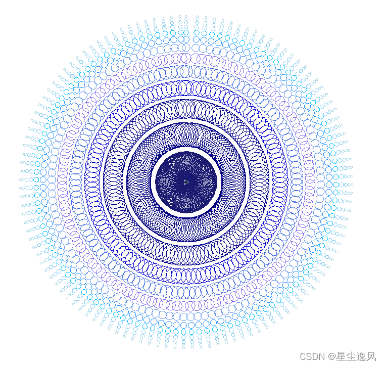
from turtle import *
speed(1000)
colormode(255)
clrs = ["MidnightBlue", "Navy", "DarkBlue", "MediumBlue", "RoyalBlue", "MediumSlateBlue", "CornflowerBlue",
        "DodgerBlue", "DeepskyBlue", "LightSkyBlue", "SkyBlue", "LightBlue"]
for j in range(120):
    cn = 0
    c = 30
    f = 70
    for i in range(12):
        pencolor(clrs[cn])
        circle(c)
        left(90)
        penup()
        forward(f)
        right(90)
        pendown()
        c = c * 0.8
        f = f * 0.8
        circle(c)
        cn = cn + 1
    penup()
    goto(0, 0)
    forward(5)
    right(3)
    pendown()
done()

随机字

在这里插入图片描述

from turtle import *
import random
strs= """
时光不老 我们不散。
心若向阳 无畏悲伤。
你若安好 便是晴天。
心有灵犀 一点就通。
人来人往 繁华似锦。
生能尽欢 死亦无憾。
花开花落 人世无常。
""".split("。")
setup(1280,720)  # 设置窗口大小
colormode(255)  # 使用的颜色模式, 整数还是小数
up()
a, b = -500, 280
goto(a,b)
bgcolor("black")
down()
def w(strs,b):
    bgcolor( 70,0,140)
    for i in range(len(strs)):
        up()
        goto(a+100*i,b)
        down()
        size =  random.randint(12,68)  # 随机字体大小
        color( random.randint(60,255),random.randint(0,255),random.randint(60,255))  # 随机字体颜色
        write(strs[i], align="center",font=("楷体",size))
for i in range(7):
    w(strs[i],b-100*i)
up()
color("#262626;")
goto(-1000,-1000)
down()
ht()
done()

tree

在这里插入图片描述

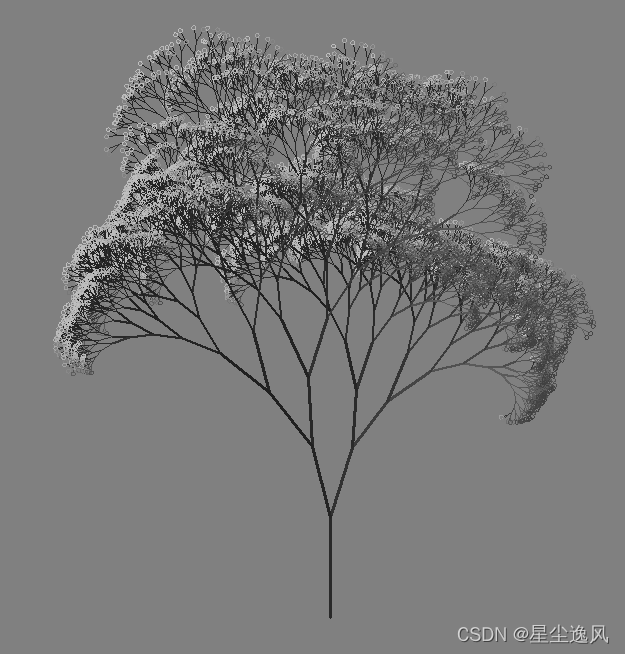
from turtle import *
from random import *
from math import *
# 递归二叉树，当到头了就画圈
def tree(n, l):
    pd()
    t = cos(radians(heading() + 45)) / 8 + 0.25
    pencolor(t, t, t)
    pensize(n / 4)
    forward(l)
    if n > 0:
        b = random() * 15 + 10
        c = random() * 15 + 10
        d = l * (random() * 0.35 + 0.6)
        right(b)
        tree(n - 1, d)
        left(b + c)
        tree(n - 1, d)
        right(c)
    else:
        right(90)
        n = cos(radians(heading() - 45)) / 4 + 0.5
        pencolor(n, n, n)
        circle(2)
        left(90)
    pu()
    backward(l)
bgcolor(0.5, 0.5, 0.5)
ht()
speed(0)
tracer(0, 0)
left(90)
pu()
backward(300)
tree(13, 100)
done()

networkx

networkx是一个用Python语言开发的图论与复杂网络建模工具，内置了常用的图与复杂网络分析算法，可以方便的进行复杂网络数据分析、仿真建模等工作。
利用networkx可以以标准化和非标准化的数据格式存储网络、生成多种随机网络和经典网络、分析网络结构、建立网络模型、设计新的网络算法、进行网络绘制等。
networkx支持创建简单无向图、有向图和多重图（multigraph）；内置许多标准的图论算法，节点可为任意数据；支持任意的边值维度，功能丰富，简单易用。
networkx以图（graph）为基本数据结构。图既可以由程序生成，也可以来自在线数据源，还可以从文件与数据库中读取。

基本流程：
　　1. 导入networkx，matplotlib包
　　2. 建立网络
　　3. 绘制网络 nx.draw()
　　4. 建立布局 pos = nx.spring_layout美化作用

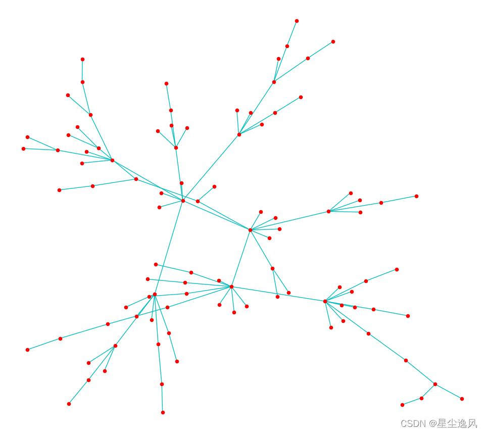
BA网络

在这里插入图片描述

import random
import networkx as nx  
import matplotlib.pyplot as plt

# G = nx.Graph()  # 创建空网络,无多重边无向图
G = nx.DiGraph()  # 无多重边有向图
# G = nx.MultiGraph()  # 有多重边无向图
# G = nx.MultiDiGraph()  # 有多重边有向图
G.add_node('a')
G.add_node('d')
G.add_nodes_from(['b', 'c']) # 从list添加节点
G.add_edge('a','db')
print(G.number_of_nodes())
print(G.number_of_edges())
G.add_nodes_from([3, 4, 5, 6, 8, 9, 10, 11, 12])  # 添加多个节点
G.add_edges_from([(3, 5), (3, 6), (6, 7)])  # 添加多条边
nx.draw(G,node_color='r')
plt.show()

G =nx.random_graphs.barabasi_albert_graph(100,1)  #生成一个BA网络,其他网络见源码
nx.draw(G,node_color=[random.random() for i in range(100)],edge_color = 'c',font_size =18,node_size=50)   #绘制网络G
plt.show()

社交网络

在这里插入图片描述

import random
import networkx as nx  
import matplotlib.pyplot as plt
import networkx.algorithms.bipartite as bipartite
G = nx.davis_southern_women_graph()
women = G.graph['top']
clubs = G.graph['bottom']
W = bipartite.projected_graph(G, women)
W = bipartite.weighted_projected_graph(G, women)
nx.draw(G, node_color="m",edge_color =[random.random() for i in range(G.number_of_edges())],font_size =10,node_size=40, with_labels=True)
plt.show()

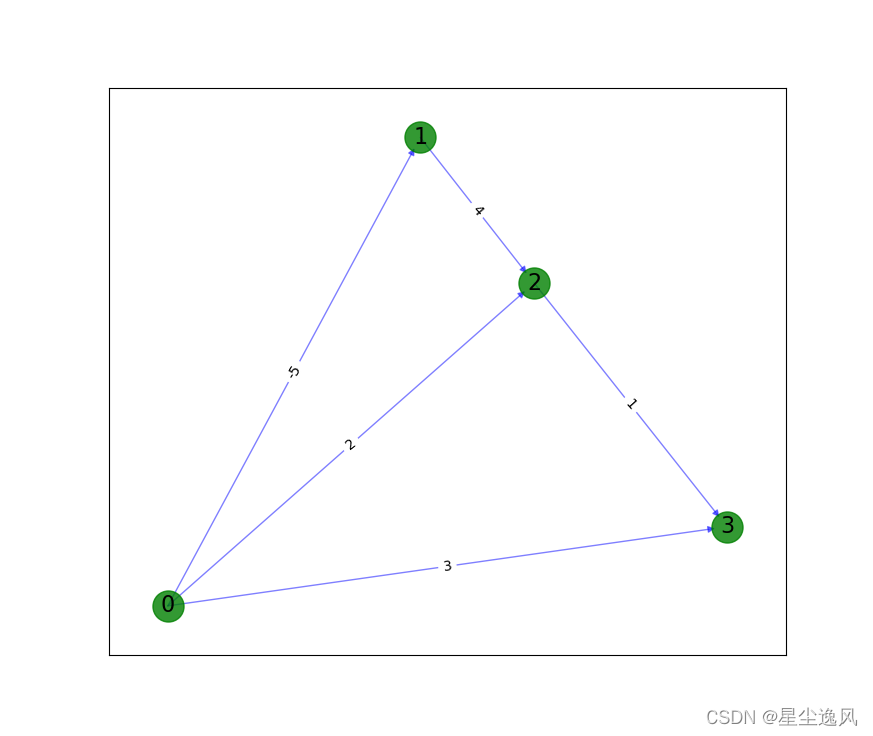
最短路径

在这里插入图片描述

import networkx as nx
import matplotlib.pyplot as plt

G = nx.DiGraph()
G.add_weighted_edges_from([('0', '3', 3), ('0', '1', -5), ('0', '2', 2), ('1', '2', 4), ('2', '3', 1)])
# 边和节点信息
edge_labels = nx.get_edge_attributes(G, 'weight')
labels = {'0': '0', '1': '1', '2': '2', '3': '3'}

# 生成节点位置
pos = nx.spring_layout(G)
# 画节点
nx.draw_networkx_nodes(G, pos, node_color='g', node_size=500, alpha=0.8)
# 画边
nx.draw_networkx_edges(G, pos, width=1.0, alpha=0.5, edge_color='b')
# 画节点的标签
nx.draw_networkx_labels(G, pos, labels, font_size=16)
# 画边权重
nx.draw_networkx_edge_labels(G, pos, edge_labels)

# 使用johnson算法计算最短路径
paths = nx.johnson(G, weight='weight')
print(paths)
plt.show()

mayavi

三维可视化
安装mayavi时不能pip，手动安装顺序为PyQt4–>Traits–>VTK–>Mayavi，找对应版本的whl

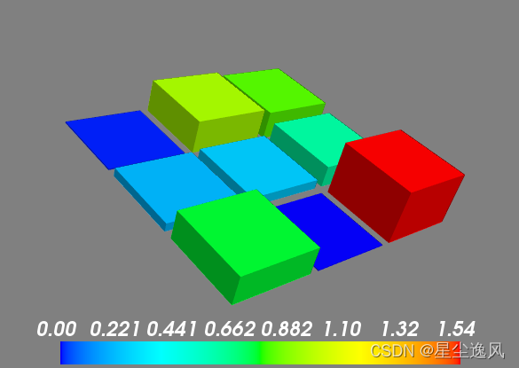
barchart

在这里插入图片描述

import random
import mayavi.mlab as mlab
import numpy as np
s = np.random.rand(3,3)
mlab.barchart(s)
mlab.vectorbar()
mlab.show()

在这里插入图片描述

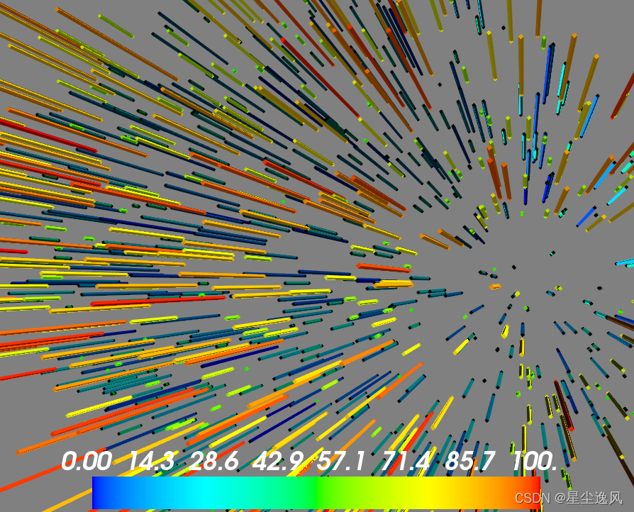
r1=[random.randint(-100,100) for i in range(1000)]
r2=[random.randint(-100,100) for i in range(1000)]
r3=[random.randint(-100,100) for i in range(1000)]
mlab.barchart(r1,r2,r3)
mlab.vectorbar()
mlab.show()

colormap

在这里插入图片描述

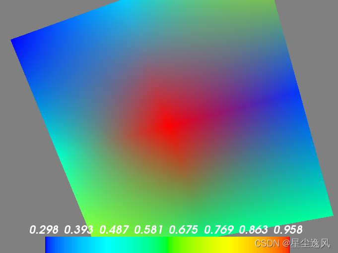
s = np.random.rand(3,3) #生成随机的3×3数组
mlab.imshow(s)
mlab.colorbar()
mlab.show()

contour3d

在这里插入图片描述

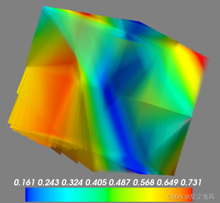
# 三维等值线图
s = np.random.rand(3,3,3)
mlab.contour3d(s, contours=60, transparent=True)
mlab.colorbar()
mlab.show()

在这里插入图片描述

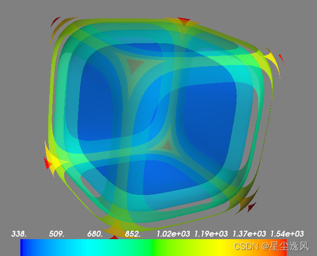
x,y,z=np.mgrid[-5.:5:64j,-5.:5:64j,-5.:5:64j]
scalars=x**4+y**4+z**4
obj=mlab.contour3d(scalars,contours=8,transparent=True)
mlab.colorbar()
mlab.show()

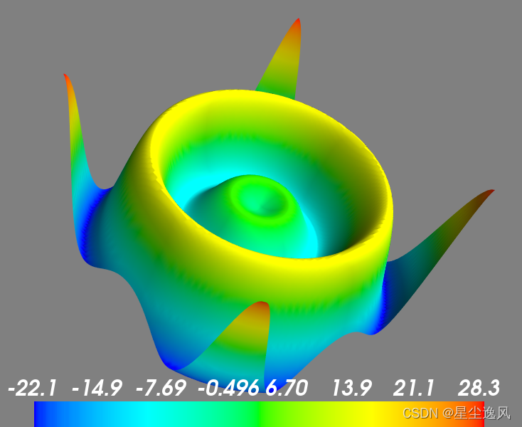
plot3d

在这里插入图片描述

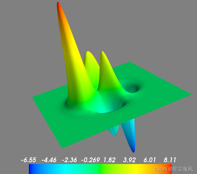
# mesh map
def peaks(x,y):  # 高斯分布
    return 3.0*(1.0-x)**2*np.exp(-(x**2) - (y+1.0)**2) - 10*(x/5.0 - x**3 - y**5) * np.exp(-x**2-y**2) - 1.0/3.0*np.exp(-(x+1.0)**2 - y**2)
y,x = np.mgrid[-5:5:700j,-5:5:700j]
z=peaks(x,y)
mlab.mesh(x,y,z)
mlab.colorbar()
mlab.show()

在这里插入图片描述

# 公式shape
x, y = np.mgrid[-10:10:100j, -10:10:100j]
r = np.sqrt(x**2 + y**2)
z = np.sin(r)*r*2
mlab.surf(z, warp_scale='auto')
mlab.colorbar()
mlab.show()

在这里插入图片描述

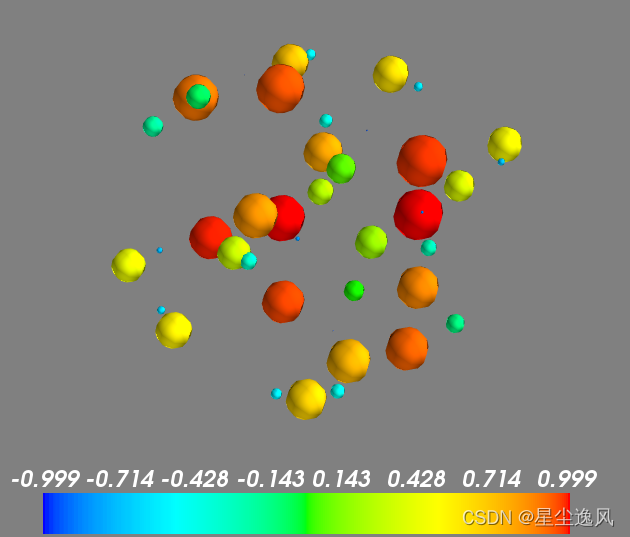
# 3D point
t=mgrid[-pi:pi:50j]
s=sin(t)  # s是每个点的大小
mlab.points3d(cos(t),sin(333*t),cos(5*t),s,mode='sphere',line_width=1)
mlab.colorbar()
mlab.show()

在这里插入图片描述

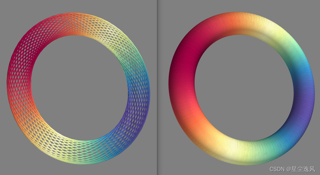
# 3D plot
n_mer, n_long = 26, 51
dphi = np.pi / 100000.0
phi = np.arange(0.0, 2 * np.pi + 0.5 * dphi, dphi)
mu = phi * n_mer
x = np.cos(mu) * (3 + np.cos(n_long * mu / n_mer) * 0.5)
y = np.sin(mu) * (3+ np.cos(n_long * mu / n_mer) * 0.5)
z = np.sin(n_long * mu / n_mer) * 0.5
mlab.plot3d(x, y, z, np.sin(mu), tube_radius=0.025, colormap='Spectral')
mlab.show()

opengl

它和opencv有点相反，cv是从图像到数据，gl是从数据到图像

星尘逸风

关注

1
点赞
踩
35

收藏

觉得还不错? 一键收藏
0
评论
一些常用的python绘图包

文章目录matplotlibseabornpyechartspygalplotlyturtlenetworkxmayaviopengl最后更新2022.02.09绘图库大全：matplotlib底层灵活可实现复杂操作seaborn是mp的上层更简单pyecharts百度的图表可视化库basemap地理地图pygal矢量图networkx网络plotly地图趋势turtle作画mayavi三维可视化opengl开放图形库其他的还有pyqtgraph、pyQT5、PIL（pill
复制链接

扫一扫