


Bag of Feature 是一种图像特征提取方法,它借鉴了文本分类的思路(Bag of Words),从图像抽象出很多具有代表性的「关键词」,形成一个字典,再统计每张图片中出现的「关键词」数量,得到图片的特征向量。Bag of Words 模型
要了解「Bag of Feature」,首先要知道「Bag of Words」。
Bag of Words 模型
「Bag of Words」 是文本分类中一种通俗易懂的策略。一般来讲,如果我们要了解一段文本的主要内容,最行之有效的策略是抓取文本中的关键词,根据关键词出现的频率确定这段文本的中心思想。这里所说的关键词,就是「Bag of words」中的 words ,它们是区分度较高的单词。根据这些 words ,我们可以很快地识别出文章的内容,并快速地对文章进行分类。而「Bag of Feature」也是借鉴了这种思路,只不过在图像中,我们抽出的不再是一个个「word」,而是图像的关键特征「Feature」,所以研究人员将它更名为「Bag of Feature」。
Bag of Feature 算法
「Bag of Feature」的本质是提出一种图像的特征表示方法。
按照「Bag of Feature」算法的思想,首先我们要找到图像中的关键词,而且这些关键词必须具备较高的区分度。实际过程中,通常会采用「SIFT」特征。有了特征之后,我们会将这些特征通过聚类算法得出很多聚类中心。这些聚类中心通常具有较高的代表性,比如,对于人脸来说,虽然不同人的眼睛、鼻子等特征都不尽相同,但它们往往具有共性,而这些聚类中心就代表了这类共性。我们将这些聚类中心组合在一起,形成一部字典(CodeBook)。
对于图像中的每个「SIFT」特征,我们能够在字典中找到最相似的聚类中心,统计这些聚类中心出现的次数,可以得到一个向量表示「直方图」,就是所谓的「Bag」。这样,对于不同类别的图片,这个向量应该具有较大的区分度,基于此,我们可以训练出一些分类模型(SVM等),并用其对图片进行分类。
Bag of features 图像检索流程
- 特征提取
- 学习视觉字典
- 针对输入特征集,根据视觉字典进行量化
- 把输入图像,根据TF-IDF转化成视觉字典的频率直方图
- 构造特征到图像的到排表,通过到排表快速索引相关图像
- 根据索引结果进行直方图匹配
提取图像特征
特征必须具有较高的区分度,而且要满足旋转不变性以及尺寸不变性等,因此,我们通常都会采用「SIFT」特征(有时为了降低计算量,也会采用其他特征,如:SURF )。「SIFT」会从图片上提取出很多特征点,每个特征点都是 128 维的向量,因此,如果图片足够多的话,我们会提取出一个巨大的特征向量库。
训练字典( visual vocabulary )
提取完特征后,我们会采用一些聚类算法对这些特征向量进行聚类。最常用的聚类算法是 k-means。至于 k-means 中的 k 如何取,要根据具体情况来确定。另外,由于特征的数量可能非常庞大,这个聚类的过程也会非常漫长。

聚类完成后,我们就得到了这 k 个向量组成的字典,这 k 个向量有一个通用的表达,叫 visual word。
图片直方图表示
上一步训练得到的字典,是为了这一步对图像特征进行量化。对于一幅图像而言,我们可以提取出大量的「SIFT」特征点,但这些特征点仍然属于一种浅层的表达,缺乏代表性。因此,这一步的目标,是根据字典重新提取图像的高层特征。
具体做法是,对于图像中的每一个「SIFT」特征,都可以在字典中找到一个最相似的 visual word,这样,我们可以统计一个 k 维的直方图,代表该图像的「SIFT」特征在字典中的相似度频率。

例如:对于上图这个图片,我们匹配图片的「SIFT」向量与字典中的 visual word,统计出最相似的向量出现的次数,最后得到这幅图片的直方图向量。
加权 BOF
TF-IDF 是通过增加权重的方法,凸显出重要的关键信息。同样的,在图像检索中,为了更精确地度量相似性,我们也在原来直方图向量的基础上,为向量的每一项增加权重。
具体的,按照上面信息检索的方法,我们需要给字典里的每个向量(visual word)设置权重。权重IDF = log(Nfj),其中,N 是图片总数,fj 表示字典向量 j 在 多少张图片上出现过。仿照上面的例子,我们可以这样理解:出现次数越少权重就越大。出现次数多的不具有特征性
假设我们按照前面 BOF 算法的过程已经得到一张图片的直方图向量 h=hj(j=0,1,…,k),那么,加权 BOF 的计算公式为:hj=(hj/∑ihi)log(Nfj)。公式右边后一部分就是上面所讲到的 IDF,而 (hj/∑ihi) 就是词频 TF。
生成代码所需模型文件
代码:
# -*- coding: utf-8 -*-
import pickle
from PCV.imagesearch import vocabulary
from PCV.tools.imtools import get_imlist
from PCV.localdescriptors import sift
#获取图像列表
imlist = get_imlist('first1000/')
nbr_images = len(imlist)
#获取特征列表
featlist = [imlist[i][:-3]+'sift' for i in range(nbr_images)]
#提取文件夹下图像的sift特征
for i in range(nbr_images):
sift.process_image(imlist[i], featlist[i])
#生成词汇
voc = vocabulary.Vocabulary('ukbenchtest')
voc.train(featlist, 1000, 10)
#保存词汇
# saving vocabulary
with open('first1000/vocabulary.pkl', 'wb') as f:
pickle.dump(voc, f)
print ('vocabulary is:', voc.name, voc.nbr_words)
用的数据集是data文件夹中的first1000图像集。

由于图片数量很多,sift特征匹配会花费很长时间

将数据模型导入数据库
使用了python中的pysqlite库,需要自己安装
代码:
# -*- coding: utf-8 -*-

import pickle

from PCV.imagesearch import imagesearch

from PCV.localdescriptors import sift

from sqlite3 import dbapi2 as sqlite

from PCV.tools.imtools import get_imlist


#获取图像列表

imlist = get_imlist('first1000/')

nbr_images = len(imlist)

#获取特征列表

featlist = [imlist[i][:-3]+'sift' for i in range(nbr_images)]


# load vocabulary

#载入词汇

with open('first1000/vocabulary.pkl', 'rb') as f:

    voc = pickle.load(f)

#创建索引

indx = imagesearch.Indexer('testImaAdd.db',voc)

indx.create_tables()

# go through all images, project features on vocabulary and insert

#遍历所有的图像,并将它们的特征投影到词汇上

for i in range(nbr_images)[:1000]:

    locs,descr = sift.read_features_from_file(featlist[i])

    indx.add_to_index(imlist[i],descr)

# commit to database

#提交到数据库

indx.db_commit()


con = sqlite.connect('testImaAdd.db')

print (con.execute('select count (filename) from imlist').fetchone())

print (con.execute('select * from imlist').fetchone())
当前目录下生成文件testlmAdd.db![]()
测试
数据放到数据库后开始测试图片的索引
代码:
# -*- coding: utf-8 -*-

import pickle

from PCV.localdescriptors import sift

from PCV.imagesearch import imagesearch

from PCV.geometry import homography

from PCV.tools.imtools import get_imlist


# load image list and vocabulary

#载入图像列表

imlist = get_imlist('first1000/')

nbr_images = len(imlist)

#载入特征列表

featlist = [imlist[i][:-3]+'sift' for i in range(nbr_images)]


#载入词汇

with open('first1000/vocabulary.pkl', 'rb') as f:

    voc = pickle.load(f)


src = imagesearch.Searcher('testImaAdd.db',voc)


# index of query image and number of results to return

#查询图像索引和查询返回的图像数

q_ind = 0

nbr_results = 20


# regular query

# 常规查询(按欧式距离对结果排序)

res_reg = [w[1] for w in src.query(imlist[q_ind])[:nbr_results]]

print ('top matches (regular):', res_reg)


# load image features for query image

#载入查询图像特征

q_locs,q_descr = sift.read_features_from_file(featlist[q_ind])

fp = homography.make_homog(q_locs[:,:2].T)


# RANSAC model for homography fitting

#用单应性进行拟合建立RANSAC模型

model = homography.RansacModel()

rank = {}


# load image features for result

#载入候选图像的特征

for ndx in res_reg[1:]:

    locs,descr = sift.read_features_from_file(featlist[ndx])  # because 'ndx' is a rowid of the DB that starts at 1

    # get matches

    matches = sift.match(q_descr,descr)

    ind = matches.nonzero()[0]

    ind2 = matches[ind]

    tp = homography.make_homog(locs[:,:2].T)

    # compute homography, count inliers. if not enough matches return empty list

    try:

        H,inliers = homography.H_from_ransac(fp[:,ind],tp[:,ind2],model,match_theshold=4)

    except:

        inliers = []

    # store inlier count

    rank[ndx] = len(inliers)


# sort dictionary to get the most inliers first

sorted_rank = sorted(rank.items(), key=lambda t: t[1], reverse=True)

res_geom = [res_reg[0]]+[s[0] for s in sorted_rank]

print ('top matches (homography):', res_geom)


# 显示查询结果

imagesearch.plot_results(src,res_reg[:8]) #常规查询

imagesearch.plot_results(src,res_geom[:8]) #重排后的结果


4.建立演示程序及Web应用
课本中用了web服务器来演示我们的成果。 使用前,我们需要先安装CherryPy包,直接运行
运行这个代码还需要一个配置文件 service.conf
![]()
代码:
# -*- coding: utf-8 -*-

import cherrypy

import pickle

import urllib

import os

from numpy import *

#from PCV.tools.imtools import get_imlist

from PCV.imagesearch import imagesearch

import random


"""

This is the image search demo in Section 7.6.

"""


class SearchDemo:


    def __init__(self):

        # 载入图像列表

        self.path = 'first1000/'

        #self.path = 'D:/python_web/isoutu/first500/'

        self.imlist = [os.path.join(self.path,f) for f in os.listdir(self.path) if f.endswith('.jpg')]

        #self.imlist = get_imlist('./first500/')

        #self.imlist = get_imlist('E:/python/isoutu/first500/')

        self.nbr_images = len(self.imlist)

        print (self.imlist)

        print (self.nbr_images)

        self.ndx = list(range(self.nbr_images))

        print (self.ndx)


        # 载入词汇

        # f = open('first1000/vocabulary.pkl', 'rb')

        with open('first1000/vocabulary.pkl','rb') as f:

            self.voc = pickle.load(f)

        #f.close()


        # 显示搜索返回的图像数

        self.maxres = 10


        # header and footer html

        self.header = """

            <!doctype html>

            <head>

            <title>Image search</title>

            </head>

            <body>

            """

        self.footer = """

            </body>

            </html>

            """


    def index(self, query=None):

        self.src = imagesearch.Searcher('testImaAdd.db', self.voc)


        html = self.header

        html += """

            <br />

            Click an image to search. <a href='?query='> Random selection </a> of images.

            <br /><br />

            """

        if query:

            # query the database and get top images

            #查询数据库,并获取前面的图像

            res = self.src.query(query)[:self.maxres]

            for dist, ndx in res:

                imname = self.src.get_filename(ndx)

                html += "<a href='?query="+imname+"'>"


                html += "<img src='"+imname+"' alt='"+imname+"' width='100' height='100'/>"

                print (imname+"################")

                html += "</a>"

            # show random selection if no query

            # 如果没有查询图像则随机显示一些图像

        else:

            random.shuffle(self.ndx)

            for i in self.ndx[:self.maxres]:

                imname = self.imlist[i]

                html += "<a href='?query="+imname+"'>"


                html += "<img src='"+imname+"' alt='"+imname+"' width='100' height='100'/>"

                print (imname+"################")

                html += "</a>"


        html += self.footer

        return html


    index.exposed = True


#conf_path = os.path.dirname(os.path.abspath(__file__))

#conf_path = os.path.join(conf_path, "service.conf")

#cherrypy.config.update(conf_path)

#cherrypy.quickstart(SearchDemo())

cherrypy.quickstart(SearchDemo(), '/', config=os.path.join(os.path.dirname(__file__), 'service.conf'))

这个是web服务器的配置文件,内容如下: 
配置文件中的第一部分为IP地址和端口,第二部分为我们的图库的地址
我的图库是在 E:/Python/pythonwatch/pcv-book-code-master/ch07/first1000/ 地址下,然后我在数据库中保存 的路径是 first1000/xxx.jpg 所以我只要将图库的地址设置成 E:/Python/pythonwatch/pcv-book-code-master/ch07 就行。
最后我们运行的时候会将我们设置的图库的地址(也就是 E:/Python/pythonwatch/pcv-book-codemaster/ch07) 和我们保存在数据库中的地址(first1000/xxx.jpg)连接起来,用于显示图片。
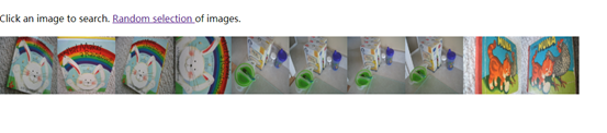
最后效果类似于这样
打开我们这只的IP地址加端口
![]()
然后就会显示我们搜索的图片


 1475
1475


 被折叠的 条评论
为什么被折叠?
被折叠的 条评论
为什么被折叠?
 到【灌水乐园】发言


